Data analysis with Pandas

Data analysis with Pandas#

Introduction#

This notebook will give a short introduction to one of the Python data analysis libraries: pandas.

Pandas is widely used in data science, machine learning, scientific computing, and many other data-intensive fields. Some of its advantages are:

data representation: easy to read, suited for data analysis
easy handling of missing data
easy to add/delete columns from pandas data structures
data alignment: intelligent automatic label-based alignment
handling large datasets
powerful grouping of data
native to Python

Pandas provides rich data structures and indexing functionality to make it easy to reshape, slice and dice, perform aggregations, and select subsets of data. Its key data structures are called the Series and DataFrame.

A Series is a one dimensional array-like object containing an array of data and an associated array of data labels, called its index.

A DataFrame is a two-dimensional tabular, column-oriented data structure with both row and column labels.

import pandas as pd
import numpy as np

Series#

A Series is a 1D array-like object containing an array of data.

first_series = pd.Series([4, 8, -10, np.nan, 2])
first_series

   4.0
   8.0
 -10.0
   NaN
   2.0
dtype: float64

The representation of first_series shows the index on the left and the values on the right. Here the default index format is used: integers 0 to N-1, N being the length of the data.

Creating a Series from a dictionary#

second_series = pd.Series({"Entry1": 0.5, "Entry2": 33.0, "Entry3": 12.0})
second_series

Entry1     0.5
Entry2    33.0
Entry3    12.0
dtype: float64

Creating a Series from a sub-selection of another Series#

third_series = pd.Series(second_series, index=["Entry1", "Entry4"])
third_series

Entry1    0.5
Entry4    NaN
dtype: float64

Adding index names#

first_series.index = ["Row1", "Row2", "Row3", "Row4", "Row5"]
first_series

Row1     4.0
Row2     8.0
Row3   -10.0
Row4     NaN
Row5     2.0
dtype: float64

Accessing information on Series#

first_series

Row1     4.0
Row2     8.0
Row3   -10.0
Row4     NaN
Row5     2.0
dtype: float64

The index object and the values can be accessed individually using:

first_series.index

Index(['Row1', 'Row2', 'Row3', 'Row4', 'Row5'], dtype='object')

first_series.values

array([  4.,   8., -10.,  nan,   2.])

The index can be used to access the values by a dictionary-like notation or by attribute

first_series.Row1

4.0

first_series["Row1"]

4.0

first_series[["Row3", "Row1"]]

Row3   -10.0
Row1     4.0
dtype: float64

# Change values stored in the Series
first_series["Row4"] = 8
first_series

Row1     4.0
Row2     8.0
Row3   -10.0
Row4     8.0
Row5     2.0
dtype: float64

Filtering, scalar multiplication or mathematical functions can be applied to a Series

# Display all positive values
first_series[first_series > 0]

Row1    4.0
Row2    8.0
Row4    8.0
Row5    2.0
dtype: float64

# Multiply all values in the Series by 2
first_series * 2

Row1     8.0
Row2    16.0
Row3   -20.0
Row4    16.0
Row5     4.0
dtype: float64

# Calculate sine of all values
np.sin(first_series)

Row1   -0.756802
Row2    0.989358
Row3    0.544021
Row4    0.989358
Row5    0.909297
dtype: float64

A Series can also be substituted into many functions that expect a dictionary.

# Check if `Row1` is in the Series
"Row1" in first_series

True

# Check if `Row9` is in the Series
"Row9" in first_series

False

DataFrame#

A DataFrame represents a spreadsheet-like data structure containing an ordered collection of columns. Each column can be a different value type: numeric, string, boolean, …

Create a DataFrame using a dictionary#

# create dictionary
first_data = {
    "Col_1": ["5", 2, "4", "7"],
    "Col_2": [
        7,
        8,
        2,
        1,
    ],
    "Col_3": [10, 4, 2, 1],
    "Col_4": [5, 6, 7, 1],
    "Col_5": [9, 9, 2, 1],
    "Col_6": [7, 8, 2, 1],
}
# convert dictionary to DataFrame
first_df = pd.DataFrame(first_data)
first_df

	Col_1	Col_2	Col_3	Col_4	Col_5	Col_6
0	5	7	10	5	9	7
1	2	8	4	6	9	8
2	4	2	2	7	2	2
3	7	1	1	1	1	1

# Display some info about the created DataFrame
first_df.info()

<class 'pandas.core.frame.DataFrame'>
RangeIndex: 4 entries, 0 to 3
Data columns (total 6 columns):
 #   Column  Non-Null Count  Dtype 
---  ------  --------------  ----- 
 0   Col_1   4 non-null      object
 1   Col_2   4 non-null      int64 
 2   Col_3   4 non-null      int64 
 3   Col_4   4 non-null      int64 
 4   Col_5   4 non-null      int64 
 5   Col_6   4 non-null      int64 
dtypes: int64(5), object(1)
memory usage: 320.0+ bytes

first_df.dtypes

Col_1    object
Col_2     int64
Col_3     int64
Col_4     int64
Col_5     int64
Col_6     int64
dtype: object

Note that Col_1 contains a mixture of integers and strings.

Viewing data#

Here is how to display the top and bottom rows of the frame

# display the top 3 rows
first_df.head(3)

	Col_1	Col_2	Col_3	Col_4	Col_5	Col_6
0	5	7	10	5	9	7
1	2	8	4	6	9	8
2	4	2	2	7	2	2

# display the bottom 2 rows
first_df.tail(2)

	Col_1	Col_2	Col_3	Col_4	Col_5	Col_6
2	4	2	2	7	2	2
3	7	1	1	1	1	1

Display the index and columns#

first_df.index

RangeIndex(start=0, stop=4, step=1)

first_df.columns

Index(['Col_1', 'Col_2', 'Col_3', 'Col_4', 'Col_5', 'Col_6'], dtype='object')

DataFrame.to_numpy() gives a NumPy representation of the data.

This can be an expensive operation when the DataFrame has columns with different data types.

DataFrame.to_numpy() does not include the index or column labels in the output.

first_df.to_numpy()

array([['5', 7, 10, 5, 9, 7],
       [2, 8, 4, 6, 9, 8],
       ['4', 2, 2, 7, 2, 2],
       ['7', 1, 1, 1, 1, 1]], dtype=object)

describe() shows a quick statistic summary of the data:

first_df.describe()

	Col_2	Col_3	Col_4	Col_5	Col_6
count	4.000000	4.000000	4.000000	4.000000	4.000000
mean	4.500000	4.250000	4.750000	5.250000	4.500000
std	3.511885	4.031129	2.629956	4.349329	3.511885
min	1.000000	1.000000	1.000000	1.000000	1.000000
25%	1.750000	1.750000	4.000000	1.750000	1.750000
50%	4.500000	3.000000	5.500000	5.500000	4.500000
75%	7.250000	5.500000	6.250000	9.000000	7.250000
max	8.000000	10.000000	7.000000	9.000000	8.000000

# to transpose the data
first_df.T

	0	1	2	3
Col_1	5	2	4	7
Col_2	7	8	2	1
Col_3	10	4	2	1
Col_4	5	6	7	1
Col_5	9	9	2	1
Col_6	7	8	2	1

Sorting#

# sorting by an axis
first_df.sort_index(axis=1, ascending=False)

	Col_6	Col_5	Col_4	Col_3	Col_2	Col_1
0	7	9	5	10	7	5
1	8	9	6	4	8	2
2	2	2	7	2	2	4
3	1	1	1	1	1	7

# sorting by values
first_df.sort_values(by=["Col_4"])

	Col_1	Col_2	Col_3	Col_4	Col_5	Col_6
3	7	1	1	1	1	1
0	5	7	10	5	9	7
1	2	8	4	6	9	8
2	4	2	2	7	2	2

Selection#

Pandas supports several types of multi-axis indexing:

.loc to choose rows and columns by label. You have to specify rows and columns based on their row and column labels.
.iloc to choose rows and columns by position. You have to specify rows and columns by their integer index.

first_df

	Col_1	Col_2	Col_3	Col_4	Col_5	Col_6
0	5	7	10	5	9	7
1	2	8	4	6	9	8
2	4	2	2	7	2	2
3	7	1	1	1	1	1

Selecting Rows#

# Select index 2 i.e. the 3rd row of the DataFrame
first_df.iloc[2]

Col_1    4
Col_2    2
Col_3    2
Col_4    7
Col_5    2
Col_6    2
Name: 2, dtype: object

If we name the index, this name can also be used to extract data

first_df.index = ["Row1", "Row2", "Row3", "Row4"]
print(f"DataFrame with named index:\n{first_df}")
print(f"\nSelection of the 3rd row:\n {first_df.loc['Row3']}")

DataFrame with named index:
     Col_1  Col_2  Col_3  Col_4  Col_5  Col_6
Row1     5      7     10      5      9      7
Row2     2      8      4      6      9      8
Row3     4      2      2      7      2      2
Row4     7      1      1      1      1      1

Selection of the 3rd row:
 Col_1    4
Col_2    2
Col_3    2
Col_4    7
Col_5    2
Col_6    2
Name: Row3, dtype: object

# Selecting several rows
# using index
first_df[0:3]

	Col_1	Col_2	Col_3	Col_4	Col_5	Col_6
Row1	5	7	10	5	9	7
Row2	2	8	4	6	9	8
Row3	4	2	2	7	2	2

# using name to select a sequence of rows
first_df.loc["Row1":"Row3"]

	Col_1	Col_2	Col_3	Col_4	Col_5	Col_6
Row1	5	7	10	5	9	7
Row2	2	8	4	6	9	8
Row3	4	2	2	7	2	2

Warning:

Note that contrary to usual Python slices, both the start and the stop are included with loc.

# using name to select rows in a different order
first_df.loc[["Row3", "Row2"]]

	Col_1	Col_2	Col_3	Col_4	Col_5	Col_6
Row3	4	2	2	7	2	2
Row2	2	8	4	6	9	8

# Selecting several rows using their positions
first_df.iloc[:, 2:4]

	Col_3	Col_4
Row1	10	5
Row2	4	6
Row3	2	7
Row4	1	1

# selecting the 4th row by position
first_df.iloc[3]

Col_1    7
Col_2    1
Col_3    1
Col_4    1
Col_5    1
Col_6    1
Name: Row4, dtype: object

Selecting columns#

# Selecting a single column. The output is a Series.
first_df["Col_4"]

Row1    5
Row2    6
Row3    7
Row4    1
Name: Col_4, dtype: int64

type(first_df["Col_4"])

pandas.core.series.Series

# Equivalent method to select a column
first_df.Col_4

Row1    5
Row2    6
Row3    7
Row4    1
Name: Col_4, dtype: int64

# Selecting several columns using their names
first_df.loc[:, "Col_2":"Col_4"]

	Col_2	Col_3	Col_4
Row1	7	10	5
Row2	8	4	6
Row3	2	2	7
Row4	1	1	1

Selecting subset#

# selecting a subset of the DataFrame using positions
first_df.iloc[1:3, 2:5]

	Col_3	Col_4	Col_5
Row2	4	6	9
Row3	2	7	2

# selecting a subset of the DataFrame using labels
first_df.loc["Row2":"Row3", "Col_3":"Col_5"]

	Col_3	Col_4	Col_5
Row2	4	6	9
Row3	2	7	2

# Getting a single value using labels
first_df.loc["Row3", "Col_4"]

# Getting a single value using positions
first_df.iloc[2, 3]

# To get faster access to a scalar
first_df.iat[2, 3]

Boolean indexing#

# Select the section of DataFrame where the values of `Col_2` are larger than 2
first_df[first_df["Col_2"] > 2]

	Col_1	Col_2	Col_3	Col_4	Col_5	Col_6
Row1	5	7	10	5	9	7
Row2	2	8	4	6	9	8

# Create a new DataFrame
second_df = pd.DataFrame(
    np.random.randn(6, 4), index=list("abcdef"), columns=list("ABCD")
)
second_df["E"] = ["one", "one", "three", "two", "three", "four"]
second_df

	A	B	C	D	E
a	-0.446545	0.070083	-0.650654	-0.310894	one
b	1.365370	0.353464	1.008604	-3.166524	one
c	0.164267	0.050503	0.577055	-1.324494	three
d	-0.497190	-0.677582	-0.874002	1.004727	two
e	-0.106611	2.023272	0.380881	-2.372564	three
f	0.339615	2.403123	-0.461630	1.052972	four

isin() can also be used for filtering

# Select row if value in 'E' column is 'three'
second_df[second_df["E"].isin(["three"])]

	A	B	C	D	E
c	0.164267	0.050503	0.577055	-1.324494	three
e	-0.106611	2.023272	0.380881	-2.372564	three

Setting#

Adding column to a DataFrame#

Create a Series to be added to second_df.

series_to_add = pd.Series([1, 2, 3, 4, 5, 6], index=["a", "b", "d", "e", "g", "h"])
series_to_add

a    1
b    2
d    3
e    4
g    5
h    6
dtype: int64

second_df["F"] = series_to_add
second_df

	A	B	C	D	E	F
a	-0.446545	0.070083	-0.650654	-0.310894	one	1.0
b	1.365370	0.353464	1.008604	-3.166524	one	2.0
c	0.164267	0.050503	0.577055	-1.324494	three	NaN
d	-0.497190	-0.677582	-0.874002	1.004727	two	3.0
e	-0.106611	2.023272	0.380881	-2.372564	three	4.0
f	0.339615	2.403123	-0.461630	1.052972	four	NaN

Note that the index is aligned: the added series has additional entries g and h and no entries for c and f. The additional entries are discarded in the DataFrame and the absence of entry is marked as NaN.

Setting values by label#

second_df.at["b", "A"] = 0
second_df

	A	B	C	D	E	F
a	-0.446545	0.070083	-0.650654	-0.310894	one	1.0
b	0.000000	0.353464	1.008604	-3.166524	one	2.0
c	0.164267	0.050503	0.577055	-1.324494	three	NaN
d	-0.497190	-0.677582	-0.874002	1.004727	two	3.0
e	-0.106611	2.023272	0.380881	-2.372564	three	4.0
f	0.339615	2.403123	-0.461630	1.052972	four	NaN

Setting values by label#

second_df.iat[1, 0] = 0
second_df

	A	B	C	D	E	F
a	-0.446545	0.070083	-0.650654	-0.310894	one	1.0
b	0.000000	0.353464	1.008604	-3.166524	one	2.0
c	0.164267	0.050503	0.577055	-1.324494	three	NaN
d	-0.497190	-0.677582	-0.874002	1.004727	two	3.0
e	-0.106611	2.023272	0.380881	-2.372564	three	4.0
f	0.339615	2.403123	-0.461630	1.052972	four	NaN

Using a NumPy array#

# Change all values in column 'C'
second_df.loc[:, "C"] = np.arange(len(second_df))
second_df

	A	B	C	D	E	F
a	-0.446545	0.070083	0.0	-0.310894	one	1.0
b	0.000000	0.353464	1.0	-3.166524	one	2.0
c	0.164267	0.050503	2.0	-1.324494	three	NaN
d	-0.497190	-0.677582	3.0	1.004727	two	3.0
e	-0.106611	2.023272	4.0	-2.372564	three	4.0
f	0.339615	2.403123	5.0	1.052972	four	NaN

Missing data#

Pandas uses numpy.nan to represent missing data. This value is by default not included in computations.

Dropping rows with missing data#

The following command will remove rows c and f because they contain one NaN value. To filter rows containing only NaN values, replace how='any' by how='all'.

second_df.dropna(axis=0, how="any", inplace=False)

	A	B	C	D	E	F
a	-0.446545	0.070083	0.0	-0.310894	one	1.0
b	0.000000	0.353464	1.0	-3.166524	one	2.0
d	-0.497190	-0.677582	3.0	1.004727	two	3.0
e	-0.106611	2.023272	4.0	-2.372564	three	4.0

Filling missing data#

The following command replaces NaN by 8.33.

second_df.fillna(value=8.33)

	A	B	C	D	E	F
a	-0.446545	0.070083	0.0	-0.310894	one	1.00
b	0.000000	0.353464	1.0	-3.166524	one	2.00
c	0.164267	0.050503	2.0	-1.324494	three	8.33
d	-0.497190	-0.677582	3.0	1.004727	two	3.00
e	-0.106611	2.023272	4.0	-2.372564	three	4.00
f	0.339615	2.403123	5.0	1.052972	four	8.33

Define a mask#

True marks the NaN values in the DataFrame.

pd.isna(second_df)

	A	B	C	D	E	F
a	False	False	False	False	False	False
b	False	False	False	False	False	False
c	False	False	False	False	False	True
d	False	False	False	False	False	False
e	False	False	False	False	False	False
f	False	False	False	False	False	True

Some of the methods to deal with missing data#

DataFrame.isna indicates missing values.

DataFrame.notna indicates existing (non-missing) values.

DataFrame.fillna replaces missing values.

Series.dropna drops missing values.

Index.dropna drops missing indices.

Operations#

Statistics#

second_df

	A	B	C	D	E	F
a	-0.446545	0.070083	0.0	-0.310894	one	1.0
b	0.000000	0.353464	1.0	-3.166524	one	2.0
c	0.164267	0.050503	2.0	-1.324494	three	NaN
d	-0.497190	-0.677582	3.0	1.004727	two	3.0
e	-0.106611	2.023272	4.0	-2.372564	three	4.0
f	0.339615	2.403123	5.0	1.052972	four	NaN

# Note that we need to discard column `E`, which contains strings, to calculate the mean
del second_df["E"]

second_df.mean()

A   -0.091077
B    0.703810
C    2.500000
D   -0.852796
F    2.500000
dtype: float64

Note that NaN values in column F have been automatically discarded.

You can also specify which axis to calculate the mean. For example, to calculate the average for each row,

second_df.mean(1)

a    0.062529
b    0.037388
c    0.222569
d    1.165991
e    1.508819
f    2.198928
dtype: float64

Apply#

Use apply to apply a function along an axis of the DataFrame

third_df = pd.DataFrame({"a": [1, 2, 3, 4, 5], "b": [7, 8, 9, 10, 11]})
third_df

	a	b
0	1	7
1	2	8
2	3	9
3	4	10
4	5	11

# calculate the square root of all elements in the DataFrame
third_df.apply(np.sqrt)

	a	b
0	1.000000	2.645751
1	1.414214	2.828427
2	1.732051	3.000000
3	2.000000	3.162278
4	2.236068	3.316625

# calculate the sum along one of the axes
third_df.apply(np.sum, axis=0)

a    15
b    45
dtype: int64

third_df.apply(np.sum, axis=1)

   8
  10
  12
  14
  16
dtype: int64

Merge#

Pandas provides several tools to easily combine Series and DataFrames.

concatenating objects with `concat()`#

Syntax:

pd.concat(objs, axis=0, join='outer', ignore_index=False, keys=None, levels=None,  
names=None, verify_integrity=False, copy=True)

Simple example:

df1 = pd.DataFrame({"A": [1, 2, 3], "B": [4, 5, 6]})
df2 = pd.DataFrame({"C": [-1, -2, -3], "D": [-4, -5, -6]})

result = pd.concat([df1, df2], join="outer")
result

	A	B	C	D
0	1.0	4.0	NaN	NaN
1	2.0	5.0	NaN	NaN
2	3.0	6.0	NaN	NaN
0	NaN	NaN	-1.0	-4.0
1	NaN	NaN	-2.0	-5.0
2	NaN	NaN	-3.0	-6.0

If join='inner', instead of getting the union of the DataFrames, we will get the intersection. For the 2 example DataFrames, the intersection is empty as shown below:

result = pd.concat([df1, df2], join="inner")
result


0
1
2
0
1
2

joining with `merge()`#

Syntax:

pd.merge(left, right, how='inner', on=None, left_on=None, right_on=None,
         left_index=False, right_index=False, sort=True,
         suffixes=('_x', '_y'), copy=True, indicator=False,
         validate=None)

Simple example:

left_df = pd.DataFrame({"key": ["0", "1"], "lval": [1, 2]})
right_df = pd.DataFrame({"key": ["0", "1", "2"], "rval": [3, 4, 5]})

left_df

	key	lval
0	0	1
1	1	2

right_df

	key	rval
0	0	3
1	1	4
2	2	5

pd.merge(left_df, right_df, on="key")

	key	lval	rval
0	0	1	3
1	1	2	4

With how='right', only the keys of the right frame are used:

pd.merge(left_df, right_df, on="key", how="right")

	key	lval	rval
0	0	1.0	3
1	1	2.0	4
2	2	NaN	5

joining on index#

left_df = pd.DataFrame(
    {"A": ["A0", "A1", "A2"], "B": ["B0", "B1", "B2"]}, index=["Key0", "Key1", "Key2"]
)


right_df = pd.DataFrame({"C": ["C0", "C2"], "D": ["D0", "D2"]}, index=["Key0", "Key2"])

result = left_df.join(right_df)
result

	A	B	C	D
Key0	A0	B0	C0	D0
Key1	A1	B1	NaN	NaN
Key2	A2	B2	C2	D2

Grouping#

“group by” is referring to a process involving one or more of the following steps:

Splitting data into groups based on some criteria
Applying a function to each group independently
Combining the results into a data structure

data_group = {
    "Detectors": [
        "Det0",
        "Det1",
        "Det2",
        "Det3",
        "Det4",
        "Det5",
        "Det6",
        "Det7",
        "Det8",
        "Det9",
        "Det10",
        "Det11",
    ],
    "GroupNb": [1, 2, 2, 3, 3, 4, 1, 1, 2, 4, 1, 2],
    "Counts": [2014, 153, 10, 5300, 123, 2000, 1075, 217, 16, 1750, 500, 800],
    "RunningOK": [
        True,
        True,
        False,
        False,
        True,
        True,
        True,
        True,
        False,
        True,
        True,
        True,
    ],
}
df_group = pd.DataFrame(data_group)

# Use 'GroupNb' to group the DataFrame
grouped = df_group.groupby("GroupNb")
for name, group in grouped:
    print(f"GroupNb: {name}")
    print(group)

GroupNb: 1
   Detectors  GroupNb  Counts  RunningOK
0       Det0        1    2014       True
6       Det6        1    1075       True
7       Det7        1     217       True
10     Det10        1     500       True
GroupNb: 2
   Detectors  GroupNb  Counts  RunningOK
1       Det1        2     153       True
2       Det2        2      10      False
8       Det8        2      16      False
11     Det11        2     800       True
GroupNb: 3
  Detectors  GroupNb  Counts  RunningOK
3      Det3        3    5300      False
4      Det4        3     123       True
GroupNb: 4
  Detectors  GroupNb  Counts  RunningOK
5      Det5        4    2000       True
9      Det9        4    1750       True

The DataFrame has been split into 4 groups according to the content of GroupNb.

Below we group the DataFrame according to RunningOK and then we sum the counts of Dets with RunningOK=True.

# Group on value of RunningOK
select_running_det = df_group.groupby(["RunningOK"])

# Sum counts of all running "Det"s
print(
    f"Total count of running Dets: {select_running_det.get_group(True)['Counts'].sum()}"
)

Total count of running Dets: 8632

# Apply several functions to the groups at once
select_running_det["Counts"].agg([np.sum, np.mean, np.std])

/tmp/ipykernel_5499/603534467.py:2: FutureWarning: The provided callable <function sum at 0x7fe7842cda20> is currently using SeriesGroupBy.sum. In a future version of pandas, the provided callable will be used directly. To keep current behavior pass the string "sum" instead.
  select_running_det["Counts"].agg([np.sum, np.mean, np.std])
/tmp/ipykernel_5499/603534467.py:2: FutureWarning: The provided callable <function mean at 0x7fe7842ce950> is currently using SeriesGroupBy.mean. In a future version of pandas, the provided callable will be used directly. To keep current behavior pass the string "mean" instead.
  select_running_det["Counts"].agg([np.sum, np.mean, np.std])
/tmp/ipykernel_5499/603534467.py:2: FutureWarning: The provided callable <function std at 0x7fe7842cea70> is currently using SeriesGroupBy.std. In a future version of pandas, the provided callable will be used directly. To keep current behavior pass the string "std" instead.
  select_running_det["Counts"].agg([np.sum, np.mean, np.std])

	sum	mean	std
RunningOK
False	5326	1775.333333	3052.452347
True	8632	959.111111	788.265571

Plotting#

# import matplotlib.pyplot as plt

# %matplotlib widget

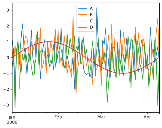
df_to_plot = pd.DataFrame(
    np.concatenate(
        (
            np.random.randn(100, 3),
            np.sin(np.linspace(0, 2 * np.pi, 100)).reshape(100, 1),
        ),
        axis=1,
    ),
    index=pd.date_range("1/1/2000", periods=100),
    columns=["A", "B", "C", "D"],
)

df_to_plot.plot();

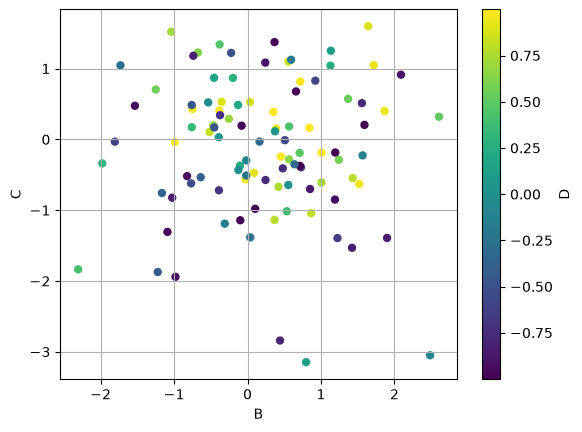
../../_images/fd9733c1718f911587fd10b13780c87597d69a7a6ea0acb6c5611c03441fa4d1.png

Plotting one column vs. another using a third column to color the points

df_to_plot.plot.scatter(x="B", y="C", c="D", grid=True, s=25);

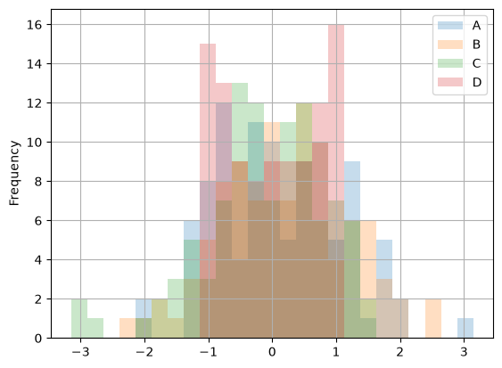
../../_images/4610ecc1bc0596fa6d3d5fb20eb4d20b9bf9ac3918a6e42eaa105769bb4ff381.png

Histograms

Histograms can be plotted using DataFrame.plot.hist() and Series.plot.hist().

help(pd.DataFrame.plot.hist)

Help on function hist in module pandas.plotting._core:

hist(self, by: 'IndexLabel | None' = None, bins: 'int' = 10, **kwargs) -> 'PlotAccessor'
    Draw one histogram of the DataFrame's columns.
    
    A histogram is a representation of the distribution of data.
    This function groups the values of all given Series in the DataFrame
    into bins and draws all bins in one :class:`matplotlib.axes.Axes`.
    This is useful when the DataFrame's Series are in a similar scale.
    
    Parameters
    ----------
    by : str or sequence, optional
        Column in the DataFrame to group by.
    
        .. versionchanged:: 1.4.0
    
           Previously, `by` is silently ignore and makes no groupings
    
    bins : int, default 10
        Number of histogram bins to be used.
    **kwargs
        Additional keyword arguments are documented in
        :meth:`DataFrame.plot`.
    
    Returns
    -------
    class:`matplotlib.AxesSubplot`
        Return a histogram plot.
    
    See Also
    --------
    DataFrame.hist : Draw histograms per DataFrame's Series.
    Series.hist : Draw a histogram with Series' data.
    
    Examples
    --------
    When we roll a die 6000 times, we expect to get each value around 1000
    times. But when we roll two dice and sum the result, the distribution
    is going to be quite different. A histogram illustrates those
    distributions.
    
    .. plot::
        :context: close-figs
    
        >>> df = pd.DataFrame(
        ...     np.random.randint(1, 7, 6000),
        ...     columns = ['one'])
        >>> df['two'] = df['one'] + np.random.randint(1, 7, 6000)
        >>> ax = df.plot.hist(bins=12, alpha=0.5)
    
    A grouped histogram can be generated by providing the parameter `by` (which
    can be a column name, or a list of column names):
    
    .. plot::
        :context: close-figs
    
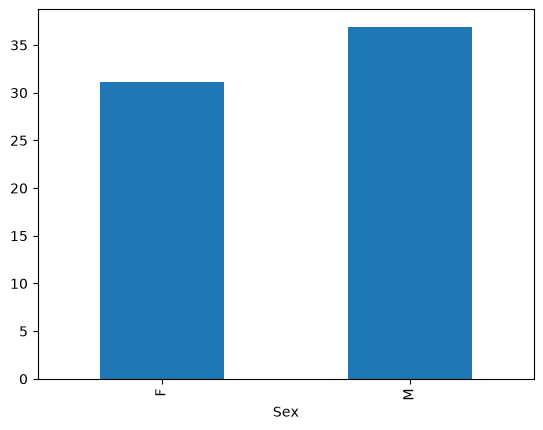
        >>> age_list = [8, 10, 12, 14, 72, 74, 76, 78, 20, 25, 30, 35, 60, 85]
        >>> df = pd.DataFrame({"gender": list("MMMMMMMMFFFFFF"), "age": age_list})
        >>> ax = df.plot.hist(column=["age"], by="gender", figsize=(10, 8))

df_to_plot.plot.hist(alpha=0.25, bins=25, grid=True);

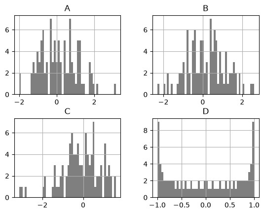
../../_images/c2f84b2d447efbe5cb717f83a34696ca44f77b2e617cd2a303f050e46dffb85e.png

DataFrame.hist() plots the histograms of the columns on multiple subplots

df_to_plot.hist(color="k", alpha=0.5, bins=50);

../../_images/5effd20f79afdc4dbdb8796a3bc1ba6b83fe9ef82434daa67e9f3b67221b666d.png

Reading and writing files#

# Create a simple DataFrame to write to files
df_to_write_to_file = pd.DataFrame(
    {
        "A": ["one", "one", "two", "three"] * 3,
        "B": ["A", "B", "C"] * 4,
        "C": ["foo", "foo", "foo", "bar", "bar", "bar"] * 2,
        "D": np.random.randn(12),
        "E": np.random.randn(12),
    }
)

df_to_write_to_file

	A	B	C	D	E
0	one	A	foo	-0.715655	0.430551
1	one	B	foo	-0.990230	-0.207351
2	two	C	foo	-1.736932	-0.613148
3	three	A	bar	0.103607	-0.712128
4	one	B	bar	-0.563637	-0.882418
5	one	C	bar	0.985882	-2.172565
6	two	A	foo	-1.374721	-0.144271
7	three	B	foo	0.454787	-0.420611
8	one	C	foo	1.782445	-1.059745
9	one	A	bar	-0.879754	-0.074875
10	two	B	bar	1.082402	1.090036
11	three	C	bar	1.454044	-1.134306

CSV#

# writing a csv file
df_to_write_to_file.to_csv("simple_file.csv")

Options can be added when saving to a .csv file. For example:

Without the index

df_to_write_to_file.to_csv('simple_file.csv', index=False)

Specify a custom delimiter for the CSV output; the default is a comma

df_to_write_to_file.to_csv('simple_file.csv',sep='\t') # Use Tab to separate data

Dealing with missing values

df_to_write_to_file.to_csv('simple_file.csv', na_rep='Unkown') # missing value saved as 'Unknown'

Specifying the precision of the data written to file

df_to_write_to_file.to_csv('simple_file.csv', float_format='%.2f')

Whether to export the column names

df_to_write_to_file.to_csv('simple_file.csv', header=False)

Select columns to be written in the .csv file. Default is None.

df_to_write_to_file.to_csv('simple_file.csv',columns=['C'])

# Reading a csv file
pd.read_csv("simple_file.csv")

	Unnamed: 0	A	B	C	D	E
0	0	one	A	foo	-0.715655	0.430551
1	1	one	B	foo	-0.990230	-0.207351
2	2	two	C	foo	-1.736932	-0.613148
3	3	three	A	bar	0.103607	-0.712128
4	4	one	B	bar	-0.563637	-0.882418
5	5	one	C	bar	0.985882	-2.172565
6	6	two	A	foo	-1.374721	-0.144271
7	7	three	B	foo	0.454787	-0.420611
8	8	one	C	foo	1.782445	-1.059745
9	9	one	A	bar	-0.879754	-0.074875
10	10	two	B	bar	1.082402	1.090036
11	11	three	C	bar	1.454044	-1.134306

HDF5#

An additional library PyTables is required to deal with HDF5 within Pandas. It can be installed within a notebook using

import sys
!{sys.executable} -m pip install tables

# Writing an HDF5 file

# df_to_write_to_file.to_hdf('simple_file.h5', 'df_to_write_to_file', format='table', mode='w')

# Reading an HDF5 file

# pd.read_hdf('simple_file.h5')

Excel#

Dealing with Excel files in Pandas requires openpyxl, xlrd. To be installed from a notebook:

import sys
!{sys.executable} -m pip install openpyxl xlrd

# Writing an Excel file

# df_to_write_to_file.to_excel('simple_file.xlsx', sheet_name='Sheet1')

# Reading an Excel file

# pd.read_excel('simple_file.xlsx', 'Sheet1')

Exercises#

The solutions can be found in the solutions folder of this repository.

How to combine series to form a dataframe?#

Combine series1 and series2 to form a DataFrame

series1 = pd.Series(["a", "b", "c", "d"])
series2 = pd.Series([1, 2, 3, 4])

Solution:

Show code cell content Hide code cell content

df = pd.DataFrame({"col1": series1, "col2": series2})
df

	col1	col2
0	a	1
1	b	2
2	c	3
3	d	4

How to stack two series vertically and horizontally?#

Stack series1 and series2 vertically and horizontally to form a dataframe.

series1 = pd.Series(range(5))
series2 = pd.Series(list("vwxyz"))

Solution:

Show code cell content Hide code cell content

# Horizontal
pd.concat([series1, series2], axis=1)

# Vertical
pd.concat([series1, series2], axis=1).T

	0	1	2	3	4
0	0	1	2	3	4
1	v	w	x	y	z

How to get the positions of items of series A in another series B?#

Get the positions of items of series2 in series1 as a list.

series1 = pd.Series([10, 3, 6, 5, 3, 1, 12, 8, 23])
series2 = pd.Series([1, 3, 5, 23])

Solution:

How to compute difference of differences between consecutive numbers of a series?#

Difference of differences between the consecutive numbers of series.

series = pd.Series([1, 3, 6, 10, 15, 21, 27, 35])

# Desired Output
# Differences:               [nan, 2.0, 3.0, 4.0, 5.0, 6.0, 6.0, 8.0]
# Difference of differences: [nan, nan, 1.0, 1.0, 1.0, 1.0, 0.0, 2.0]

Solution:

How to check if a dataframe has any missing values?#

Check if df has any missing values.

df = pd.DataFrame(np.random.randn(6, 4), index=list("abcdef"), columns=list("ABCD"))
df["E"] = [0.5, np.nan, -0.33, np.nan, 3.14, 8]
df

	A	B	C	D	E
a	0.324884	-1.203289	0.498207	1.261113	0.50
b	-0.863527	0.653668	0.570762	-0.880349	NaN
c	0.970973	0.832854	1.268782	-0.632254	-0.33
d	-0.333298	-0.985844	1.448454	-0.352328	NaN
e	1.804729	-0.568621	1.588207	-1.159730	3.14
f	1.199277	-0.701474	1.824473	-1.193692	8.00

Solution:

Playing with `groupby` and csv files#

load the csv file biostats.csv to a users DataFrame
determine the average, minimum and maximum ages per gender
determine the average weight of people over 35 years of age

df = pd.read_csv(
    "https://people.sc.fsu.edu/~jburkardt/data/csv/biostats.csv", skipinitialspace=True
)

Solution:

# Average age per gender
print("Average age per gender", df.groupby("Sex")["Age"].mean())

# One can also plot the result
df.groupby("Sex")["Age"].mean().plot(kind="bar")

print()

# min max age per gender
print("Minimum age by gender:", df.groupby("Sex")["Age"].min())
print("Maximum age by gender:", df.groupby("Sex")["Age"].max())

# Other solution: Calculate average, mean and max at once
display(df.groupby("Sex")["Age"].agg([np.mean, np.min, np.max]))

# Average weight and height of people over 35 years of age
print("35 year olds:")
users[users.Age > 35].loc[:, "Height (in)":"Weight (lbs)"].mean()

Average age per gender Sex
F    31.142857
M    36.909091
Name: Age, dtype: float64

Minimum age by gender: Sex
F    23
M    29
Name: Age, dtype: int64
Maximum age by gender: Sex
F    47
M    53
Name: Age, dtype: int64

/tmp/ipykernel_5499/1571231152.py:14: FutureWarning: The provided callable <function mean at 0x7fe7842ce950> is currently using SeriesGroupBy.mean. In a future version of pandas, the provided callable will be used directly. To keep current behavior pass the string "mean" instead.
  display(df.groupby("Sex")["Age"].agg([np.mean, np.min, np.max]))
/tmp/ipykernel_5499/1571231152.py:14: FutureWarning: The provided callable <function min at 0x7fe7842ce170> is currently using SeriesGroupBy.min. In a future version of pandas, the provided callable will be used directly. To keep current behavior pass the string "min" instead.
  display(df.groupby("Sex")["Age"].agg([np.mean, np.min, np.max]))
/tmp/ipykernel_5499/1571231152.py:14: FutureWarning: The provided callable <function max at 0x7fe7842ce050> is currently using SeriesGroupBy.max. In a future version of pandas, the provided callable will be used directly. To keep current behavior pass the string "max" instead.
  display(df.groupby("Sex")["Age"].agg([np.mean, np.min, np.max]))

	mean	min	max
Sex
F	31.142857	23	47
M	36.909091	29	53

35 year olds:

---------------------------------------------------------------------------
NameError                                 Traceback (most recent call last)
Cell In[103], line 18
     16 # Average weight and height of people over 35 years of age
     17 print("35 year olds:")
---> 18 users[users.Age > 35].loc[:, "Height (in)":"Weight (lbs)"].mean()

NameError: name 'users' is not defined

../../_images/acfe9990948bc2cf2c3ea38150f4e2f14deadf02c579146c362d8bff9844afff.png

References#

https://pandas.pydata.org/

https://pandas.pydata.org/pandas-docs/stable/user_guide/10min.html

Exercises:
https://www.w3resource.com/python-exercises/pandas/index.php
guipsamora/pandas_exercises

CSV files:
https://people.sc.fsu.edu/~jburkardt/data/csv/csv.html

Data analysis with Pandas

Contents

Data analysis with Pandas#

Introduction#

Series#

Creating a Series from a dictionary#

Creating a Series from a sub-selection of another Series#

Adding index names#

Accessing information on Series#

DataFrame#

Create a DataFrame using a dictionary#

Viewing data#

Display the index and columns#

Sorting#

Selection#

Selecting Rows#

Selecting columns#

Selecting subset#

Boolean indexing#

Setting#

Adding column to a DataFrame#

Setting values by label#

Setting values by label#

Using a NumPy array#

Missing data#

Dropping rows with missing data#

Filling missing data#

Define a mask#

Some of the methods to deal with missing data#

Operations#

Statistics#

Apply#

Merge#

concatenating objects with concat()#

joining with merge()#

joining on index#

Grouping#

Plotting#

Reading and writing files#

CSV#

HDF5#

Excel#

Exercises#

How to combine series to form a dataframe?#

How to stack two series vertically and horizontally?#

How to get the positions of items of series A in another series B?#

How to compute difference of differences between consecutive numbers of a series?#

How to check if a dataframe has any missing values?#

Playing with groupby and csv files#

References#

concatenating objects with `concat()`#

joining with `merge()`#

Playing with `groupby` and csv files#