Bayesian Model Selection

Occasionally, there is more than one mathematical model that may describe the system that you have measured. Within the Bayesian paradigm, we can discern between different models through the quantification of the Bayesian evidence (the denominator in (6)), which we will now refer to as \(P(B|M)\) (previously the \(M\) was removed for convenience). The evidence is found by integrating over the product of the likelihood and the prior:

(7)\[P(B|M) = \int P(B|A,M) P(A|M)\;dA\]

This means that, as more parameters are included in the model, there is a weighting against these models, as another dimension is included in the integral. This can be used to ensure that we do not overfit our data with an overly complex model.

Given the potentially large dimensionality of the integral that needs to be computed to estimate \(P(B|M)\), straight forward numerical calculation is typically unfeasible. Therefore, it is necessary to use a more efficient approach, one of the most popular of these is nested sampling, which we can take advantage of in Python using the package dynesty. Unlike MCMC, it is not necessary to have a good initial guess of the parameters for nested sampling. Therefore, below it is only necessary that we construct our data, model, and parameters.

from easyCore import np
from easyCore.Objects.Variable import Parameter
from easyCore.Objects.ObjectClasses import BaseObj
from easyCore.Fitting.Fitting import Fitter

np.random.seed(123)

a_true = -0.9594
b_true = 7.294
c_true = 3.102

N = 25
x = np.linspace(0, 10, N)
yerr = 1 + 1 * np.random.rand(N)
y = a_true * x ** 2 + b_true * x + c_true
y += np.abs(y) * 0.1 * np.random.randn(N)

a = Parameter(name='a', value=a_true, fixed=False, min=-5.0, max=0.5)
b = Parameter(name='b', value=b_true, fixed=False, min=0, max=10)
c = Parameter(name='c', value=c_true, fixed=False, min=-20, max=50)

def math_model(x: np.ndarray) -> np.ndarray:
    """
    Mathematical model for a quadratic. 
    
    :x: values to calculate the model over. 
    
    :return: model values.
    """
    return a.raw_value * x ** 2 + b.raw_value * x + c.raw_value

quad = BaseObj(name='quad', a=a, b=b, c=c)
f = Fitter(quad, math_model)

The log-likelihood function is identical to the MCMC example.

from scipy.stats import multivariate_normal

mv = multivariate_normal(mean=y, cov=np.diag(yerr ** 2))

def log_likelihood(theta: np.ndarray, x: np.ndarray) -> float:
    """
    The log-likelihood function for the data given a model. 

    :theta: the model parameters.
    :x: the value over which the model is computed.

    :return: log-likelihood for the given parameters.
    """
    a.value, b.value, c.value = theta
    model = f.evaluate(x)
    logl = mv.logpdf(model)
    return logl

However, the prior probability function is set up in a slightly different way, calculating the percent point function (ppf) instead of the probability density function (pdf).

from typing import List
from scipy.stats import uniform

priors = []
for p in f.fit_object.get_parameters():
    priors.append(uniform(loc=p.min, scale=p.max - p.min))

def prior(u: np.ndarray) -> List[float]:
    """
    The percent point function for the prior distributions. 
    
    :u: the model parameters.
    
    :return: list of ppfs for the given parameters and priors.
    """
    return [p.ppf(u[i]) for i, p in enumerate(priors)]

Then, similar to the MCMC example, we use the external package to perform the sampling. Note that nested sampling runs until some acceptance criterion is reached, not for a given number of samples. For this toy problem, this should be relatively fast (~1 minute to complete).

from dynesty import NestedSampler

ndim = len(f.fit_object.get_parameters())

sampler = NestedSampler(log_likelihood, prior, ndim, logl_args=[x])

sampler.run_nested(print_progress=False)

The parameter that we are interested in is the Bayesian evidence, which is called logz in dynesty, which can be obtained from the results object. However, the nested sampling approach is an iterative process that gradually moves closed to an estimate of logz, therefore, this object is a list of floats. We are interested in the final value.

results = sampler.results
print('P(D|M) = ', results.logz[-1])

P(D|M) =  -56.82486791340576

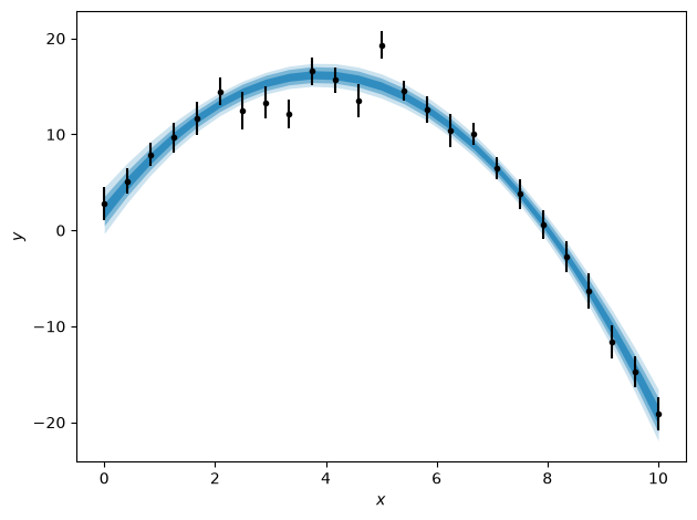
Finally, similar plots to those for MCMC can be produced by obtaining the samples from the results.

import matplotlib.pyplot as plt
import corner

flat_samples = results.samples_equal()

fig = corner.corner(flat_samples, labels=['a', 'b', 'c'])

credible_intervals = [[16, 84], [2.5, 97.5], [0.15, 99.85]]
alpha = [0.6, 0.4, 0.2]
distribution = flat_samples[:, 0] * x[:, np.newaxis] ** 2 + flat_samples[:, 1] * x[:, np.newaxis] + flat_samples[:, 2]

plt.errorbar(x, y, yerr, marker='.', ls='', color='k')
for i, ci in enumerate(credible_intervals):
    plt.fill_between(x,
                     *np.percentile(distribution, ci, axis=1),
                     alpha=alpha[i],
                     color='#0173B2',
                     lw=0)
plt.xlabel('$x$')
plt.ylabel('$y$')
plt.show()

This evidence can then be compared with that for a more complex model with more parameters. For example, the code below implements a model with the cubic form

(8)\[ y = \alpha x ^ 3 + \beta x ^ 2 + \gamma x + \delta, \]

where \(\alpha\), \(\beta\), \(\gamma\), and \(\delta\) are the parameters to be optimised.

alpha = Parameter(name='alpha', value=3, fixed= False, min=-5.0, max=5.0)
beta = Parameter(name='beta', value=a.raw_value, fixed=False, min=-5.0, max=0.5)
gamma = Parameter(name='gamma', value=b.raw_value, fixed=False, min=0, max=10)
delta = Parameter(name='delta', value=c.raw_value, fixed=False, min=-20, max=50)

def math_model(x: np.ndarray) -> np.ndarray:
    """
    A mathematical implementation of a cubic model. 
    
    :x: values to calculate the model for.
    
    :return: model values.
    """
    return alpha.raw_value * x ** 3 + beta.raw_value * x ** 2 + gamma.raw_value * x + delta.raw_value

cubic = BaseObj(name='cubic', alpha=alpha, beta=beta, gamma=gamma, delta=delta)
f_cubic = Fitter(cubic, math_model)

A new log-likelihood and prior function are required for this new model.

def log_likelihood_cubic(theta, x):
    """
    The log-likelihood function for the data given a more complex model. 

    :theta: the model parameters.
    :x: the value over which the model is computed.

    :return: log-likelihood for the given parameters.
    """
    alpha.value, beta.value, gamma.value, delta.value = theta
    model = f_cubic.evaluate(x)
    logl = mv.logpdf(model)
    return logl

priors_cubic = []
for p in f_cubic.fit_object.get_parameters():
    priors_cubic.append(uniform(loc=p.min, scale=p.max - p.min))

def prior_cubic(u):
    return [p.ppf(u[i]) for i, p in enumerate(priors_cubic)]

And as above, the nested sampling algorithm is run.

ndim = len(f_cubic.fit_object.get_parameters())

sampler_cubic = NestedSampler(log_likelihood_cubic, prior_cubic, ndim, logl_args=[x])

sampler_cubic.run_nested(print_progress=False)

The evidence between the two models can then be compared.

results_cubic = sampler_cubic.results

print('quadratic evidence = ', results.logz[-1])
print('cubic evidence = ', results_cubic.logz[-1])

quadratic evidence =  -56.82486791340576
cubic evidence =  -61.43026719303195

The decrease in Bayesian evidence with the introduction of another parameter indicates that using the cubic model would be overfitting the data and should be avoided in favour of the simpler model.