Introduction to Scipp#
Multi-dimensional arrays with labeled dimensions and physical units
scipp.github.io
Scipp is an open-source library developed by ESS for handling, manipulating and visualizing multi-dimensional data arrays.
It enriches raw NumPy-like arrays by adding named dimensions and associated coordinates. In addition, it supports
Physical units which are handled in arithmetic operations
Histograms, i.e., bin-edge axes, which are by 1 longer than the data extent
Propagation of uncertainties
#!pip install jupyterquiz
%matplotlib inline
import numpy as np
import scipp as sc
import matplotlib.pyplot as plt

from scipp_utils import quiz, plot, scatter, fetch_data

rng = np.random.default_rng(seed=1234)
1. Labeled dimensions: why do we need them?#
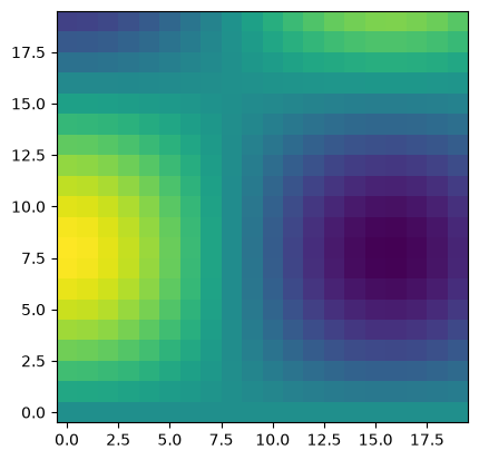
Say we have a 2D rectangular array of data
ny, nx = 10, 20
a = np.sin(np.arange(ny) / (ny / 4)).reshape((-1, 1)) * np.cos(np.arange(nx) / (ny / 4))
a.shape
(10, 20)
that looks like
plot(a)
The task is now to slice out row number 4. Because of the shape of the array, we know that the row dimension is the smallest, so we slice the first dimension of the 2D array:
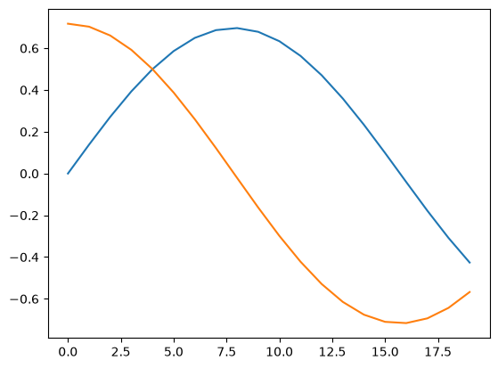
# Slice out row number 4
plot(a[4, :])
We can’t always deduce from the shape#
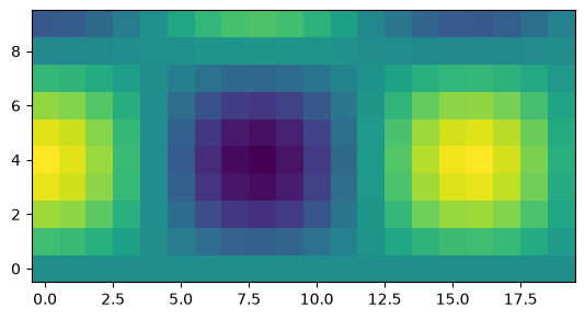
Now say we have an array which has a square shape:
ny, nx = 20, 20
a = np.sin(np.arange(ny) / (ny / 4)).reshape((-1, 1)) * np.cos(np.arange(nx) / (ny / 4))
a.shape
(20, 20)
plot(a)
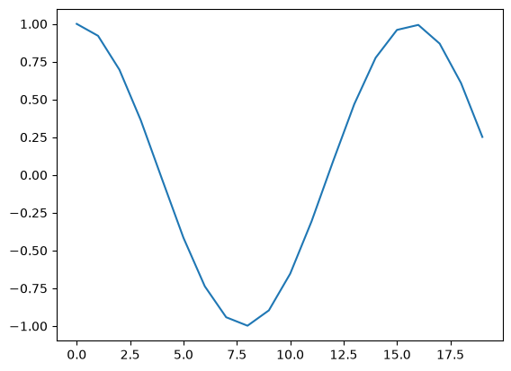
Do we slice the first or the second index of the 2D array?
# Not always obvious which dimension is which
plot(a[:, 4], a[4, :])
The situation gets worse with more dimensions#
Say we now have an array that has 4 dimensions: x, y, z, t (in that order, maybe?, or is it z, y, x, t, or t, x, y, z?)
a = np.random.random([20] * 4)
a.shape
(20, 20, 20, 20)
Quiz time!
quiz(1)
Introducing labeled dimensions#
![]()
![]()
Xarray introduced labels to multi-dimensional Numpy arrays.
“real-world datasets are usually more than just raw numbers; they have labels which encode information about how the array values map to locations in space, time, etc.”
We have embraced, and to a large extent copied, the Xarray mechanism.
var = sc.array(dims=["x", "y", "z", "time"], values=a)
var
- (x: 20, y: 20, z: 20, time: 20)float64𝟙0.060, 0.801, ..., 0.756, 0.698
Values:
array([[[[5.96179560e-02, 8.00543799e-01, 7.44652328e-01, ...,
          2.76273130e-01, 2.00141692e-01, 9.55636810e-01],
         [8.49731527e-01, 6.18912189e-02, 2.12367928e-01, ...,
          4.39195240e-01, 4.74872164e-01, 6.19476565e-01],
         [9.21396623e-01, 8.87026201e-01, 3.61104966e-01, ...,
          2.70082698e-01, 4.89357259e-01, 2.18176330e-01],
         ...,
         [3.35696575e-01, 6.79710210e-02, 9.53829025e-01, ...,
          2.63937937e-02, 6.21419834e-01, 7.55011887e-01],
         [5.97845363e-01, 7.98294966e-01, 3.18045888e-01, ...,
          5.45623409e-01, 9.54004594e-01, 1.21825159e-01],
         [1.89191606e-02, 9.99081380e-02, 6.77057890e-01, ...,
          3.01904414e-02, 6.42107798e-01, 2.96986114e-01]],

        [[4.20295391e-01, 9.87494183e-01, 8.20648387e-01, ...,
          4.36686683e-01, 9.71976695e-01, 3.90264673e-02],
         [7.20447419e-01, 6.62524181e-01, 4.92354912e-03, ...,
          4.49967229e-01, 8.20431848e-01, 4.20808823e-01],
         [2.12316315e-01, 1.46228453e-01, 1.12435895e-01, ...,
          7.24100102e-01, 5.25698835e-01, 2.09932846e-02],
         ...,
         [2.77447806e-01, 1.45529347e-03, 1.65281855e-01, ...,
          7.72447635e-01, 6.86461735e-02, 5.03439744e-01],
         [2.55682935e-01, 8.26621615e-03, 7.33213286e-01, ...,
          7.89257568e-01, 3.80726128e-01, 4.22881476e-02],
         [2.56670794e-01, 4.65490541e-01, 1.53881557e-01, ...,
          8.72299823e-01, 5.57879875e-01, 5.60616334e-01]],

        [[5.22114582e-01, 6.73107334e-01, 9.04035681e-01, ...,
          8.08400336e-01, 8.61671740e-01, 1.00353007e-01],
         [7.81229934e-01, 6.20966787e-01, 5.44046292e-01, ...,
          5.44659592e-01, 2.09995160e-01, 4.86686176e-01],
         [3.68754054e-01, 8.23349811e-01, 6.17073667e-01, ...,
          7.98005310e-01, 2.05532848e-01, 3.08798224e-01],
         ...,
         [2.03875479e-01, 3.46686685e-01, 3.65596105e-02, ...,
          5.96098858e-01, 9.65281153e-01, 4.18252225e-01],
         [8.97459941e-01, 6.99884613e-01, 9.78278686e-01, ...,
          4.36801804e-01, 8.06889163e-01, 2.53374911e-01],
         [9.14334913e-01, 6.29771626e-01, 1.00181194e-01, ...,
          6.09645950e-01, 5.51125236e-03, 3.63693057e-01]],

        ...,

        [[2.33618708e-01, 2.99585486e-01, 4.02925657e-03, ...,
          3.04532927e-02, 8.14891394e-01, 6.91643884e-01],
         [8.48700272e-01, 8.30837108e-01, 4.58289959e-02, ...,
          1.60864882e-02, 1.23725216e-01, 4.76952167e-01],
         [2.79391128e-01, 9.48575986e-01, 3.38335291e-01, ...,
          4.62223694e-01, 6.56198472e-01, 3.31292839e-01],
         ...,
         [3.70903985e-01, 6.47555268e-01, 7.62248340e-01, ...,
          8.06065009e-01, 2.33577016e-01, 2.38454629e-02],
         [9.57082856e-01, 8.75193230e-01, 3.59929193e-01, ...,
          7.47304138e-02, 6.35490452e-02, 9.90178312e-01],
         [9.75719025e-01, 8.46685760e-01, 4.84421018e-01, ...,
          7.41054273e-01, 1.85770993e-01, 3.33488313e-01]],

        [[8.64157965e-01, 5.05137269e-01, 6.41513650e-01, ...,
          1.58378663e-01, 8.10378203e-01, 8.73683041e-01],
         [2.97041424e-01, 2.05784701e-01, 5.93832415e-01, ...,
          6.23073736e-02, 8.59905775e-01, 6.27811237e-01],
         [3.11047110e-01, 3.12116756e-01, 8.93866806e-01, ...,
          5.83594042e-01, 5.96883660e-01, 6.54499449e-01],
         ...,
         [4.58646176e-01, 9.54963533e-01, 4.40299534e-01, ...,
          2.20320593e-01, 1.35605315e-01, 6.69231346e-01],
         [4.14661313e-01, 4.09477261e-01, 3.40517676e-01, ...,
          2.28390788e-01, 6.14334873e-01, 2.59705645e-01],
         [4.35418873e-01, 4.31033545e-01, 3.80137106e-01, ...,
          9.81483627e-02, 5.66193815e-01, 3.87848569e-01]],

        [[6.67657903e-01, 8.00528946e-01, 8.99624565e-01, ...,
          1.87430279e-02, 6.74326114e-01, 8.49155845e-01],
         [3.88745225e-02, 5.06882432e-01, 8.47096709e-01, ...,
          7.32961613e-01, 6.89920859e-02, 9.47650553e-01],
         [5.51248731e-01, 3.40625662e-01, 3.55189183e-01, ...,
          6.05629654e-01, 2.77197684e-01, 1.29715863e-01],
         ...,
         [1.58207511e-02, 8.39537356e-01, 3.79553686e-01, ...,
          1.66636617e-01, 3.80015715e-01, 2.10321806e-01],
         [2.94179288e-01, 7.97393847e-01, 4.91380965e-01, ...,
          2.01830711e-01, 4.36722294e-01, 3.05953255e-01],
         [6.49069953e-01, 8.97005971e-01, 8.17292345e-01, ...,
          1.98709807e-01, 7.59956843e-01, 2.15149649e-01]]],


       [[[7.28109730e-02, 9.21051165e-01, 3.93790641e-01, ...,
          5.74847813e-01, 6.99231467e-01, 6.03654028e-01],
         [5.87796648e-01, 8.81729735e-02, 4.94903694e-01, ...,
          9.46413102e-01, 6.16490979e-01, 3.61352141e-01],
         [1.86827677e-01, 7.14230119e-01, 4.84016484e-01, ...,
          5.52559847e-01, 7.20353403e-01, 6.85344111e-01],
         ...,
         [3.26735181e-01, 2.86066208e-01, 6.70866121e-01, ...,
          7.73322941e-02, 5.00190165e-03, 4.01530720e-01],
         [8.47040598e-01, 3.43190142e-01, 7.34788885e-01, ...,
          7.92561751e-01, 9.48004574e-01, 4.29525570e-01],
         [1.41865595e-01, 9.42972215e-01, 9.74391903e-01, ...,
          6.64222788e-01, 5.52339770e-01, 6.26063852e-01]],

        [[6.90681508e-01, 6.22894266e-01, 5.88999526e-01, ...,
          8.93965379e-01, 2.60844727e-01, 9.78754668e-01],
         [8.35713581e-01, 9.49968640e-01, 3.67331319e-01, ...,
          9.11453496e-01, 8.56261939e-01, 6.98277618e-01],
         [9.93575437e-01, 1.36476191e-01, 9.47497059e-01, ...,
          5.80883150e-01, 6.89848683e-01, 3.92060174e-01],
         ...,
         [5.24950033e-01, 5.22153906e-01, 3.99523829e-01, ...,
          5.72316768e-01, 3.48772830e-01, 8.47124743e-01],
         [2.36664474e-01, 9.36492700e-01, 5.76650505e-01, ...,
          1.57004517e-01, 5.27522335e-01, 3.78603861e-01],
         [7.61387429e-01, 1.76472913e-01, 5.18803772e-01, ...,
          4.76586123e-01, 1.00556256e-01, 7.59131350e-01]],

        [[3.55600920e-01, 7.33047173e-01, 1.31852568e-01, ...,
          3.39746770e-01, 7.17724923e-01, 9.28040292e-01],
         [9.48175292e-02, 4.05919992e-02, 5.35023625e-01, ...,
          7.51784706e-01, 1.51997590e-02, 1.43308150e-01],
         [2.83861833e-01, 3.44720924e-01, 8.80113950e-01, ...,
          9.17671157e-01, 6.06176908e-01, 7.08130158e-02],
         ...,
         [7.53781949e-02, 5.84227386e-01, 8.88848062e-01, ...,
          2.05459007e-01, 5.35225048e-01, 3.39457539e-02],
         [4.76648114e-01, 1.21525686e-01, 5.45533052e-01, ...,
          4.08816626e-01, 2.95381441e-01, 5.60258585e-01],
         [2.14152859e-01, 2.75470496e-02, 6.57107287e-01, ...,
          4.22635780e-01, 5.30978201e-01, 6.72491007e-01]],

        ...,

        [[9.65167307e-01, 6.44313663e-01, 9.85023231e-01, ...,
          1.46311287e-01, 3.14336320e-01, 2.45802549e-01],
         [7.18906792e-02, 2.48618844e-01, 8.48420062e-01, ...,
          8.41162803e-01, 1.35579198e-01, 1.16655349e-01],
         [5.17084156e-01, 1.58418303e-01, 8.40375364e-02, ...,
          5.13684523e-03, 4.56765277e-01, 7.35017120e-01],
         ...,
         [3.77670444e-01, 5.23102653e-01, 3.96180710e-01, ...,
          3.51434970e-01, 9.67456015e-02, 4.48185255e-01],
         [7.30322017e-01, 2.70669812e-01, 6.09676607e-01, ...,
          1.95371477e-02, 3.94442173e-01, 6.59558465e-01],
         [7.10209903e-01, 4.54782791e-01, 9.99005759e-01, ...,
          2.66252303e-01, 5.15144971e-01, 5.87961888e-01]],

        [[6.96886890e-01, 8.18355455e-01, 7.98832628e-01, ...,
          7.33178683e-01, 8.19568694e-01, 1.30158712e-01],
         [2.66410985e-01, 7.92664582e-01, 4.47839639e-01, ...,
          3.61453324e-01, 8.81198567e-01, 9.53242857e-03],
         [9.62278663e-01, 4.23970558e-01, 1.69631265e-01, ...,
          6.56307522e-01, 5.26152931e-01, 3.82890432e-01],
         ...,
         [4.14001223e-01, 5.21975286e-01, 6.78723444e-01, ...,
          3.97313694e-01, 3.55004429e-01, 2.09062704e-01],
         [2.68376383e-01, 2.63342691e-01, 8.15959657e-01, ...,
          4.51555055e-01, 7.12399236e-01, 8.72144881e-01],
         [3.17168992e-01, 5.45192072e-01, 1.69366922e-01, ...,
          1.65506413e-01, 6.66775472e-01, 6.76904350e-01]],

        [[6.93847193e-02, 5.81781402e-01, 3.10731668e-01, ...,
          3.20693344e-01, 4.37736615e-01, 5.59868664e-01],
         [4.56187254e-01, 3.80882460e-01, 2.45742991e-01, ...,
          2.25175134e-01, 6.43148253e-01, 3.63488702e-01],
         [3.43372351e-01, 7.04809704e-02, 5.46953966e-01, ...,
          1.73400981e-01, 3.35618128e-02, 7.20781686e-01],
         ...,
         [9.26106963e-01, 7.40720487e-01, 3.56536256e-01, ...,
          5.86077256e-01, 3.56492677e-01, 5.98154470e-01],
         [2.78310928e-01, 9.33521192e-01, 3.73985504e-01, ...,
          9.15110148e-01, 4.14613269e-01, 4.57045668e-01],
         [6.65591724e-01, 6.46478930e-01, 9.49733899e-01, ...,
          5.30801225e-01, 3.18127458e-01, 8.42048144e-01]]],


       [[[2.04507754e-01, 6.95137217e-01, 8.40227943e-01, ...,
          6.75842069e-01, 2.87052802e-01, 5.41188092e-01],
         [1.86909271e-01, 7.84281422e-02, 9.41365821e-01, ...,
          4.34965387e-02, 3.61044887e-01, 9.59270033e-01],
         [2.08503434e-01, 2.54483642e-01, 5.12341451e-01, ...,
          3.70434788e-02, 3.94525434e-01, 9.06919828e-01],
         ...,
         [3.15803756e-01, 4.89704418e-01, 8.95541569e-01, ...,
          6.65009214e-01, 3.16367833e-01, 4.28899627e-01],
         [8.53315722e-01, 7.86734413e-01, 8.59602026e-01, ...,
          6.61801574e-01, 1.90286718e-01, 9.66902193e-01],
         [6.13623645e-01, 2.81971870e-01, 7.13430962e-01, ...,
          1.59818541e-01, 8.17333505e-01, 2.29790335e-01]],

        [[9.26191303e-01, 3.69123323e-01, 4.39946522e-01, ...,
          2.41434285e-02, 4.62672280e-01, 8.33202573e-01],
         [4.27107868e-02, 9.50584907e-01, 7.18422207e-01, ...,
          1.84354904e-01, 7.48255846e-01, 4.77222177e-01],
         [4.17792294e-02, 9.15344883e-01, 7.53830616e-03, ...,
          4.15659327e-01, 1.28588306e-01, 2.70809481e-02],
         ...,
         [6.97362794e-01, 4.97741486e-01, 5.87999872e-01, ...,
          3.57671574e-01, 8.73368225e-01, 5.43381249e-01],
         [4.04121419e-01, 1.54848388e-01, 6.63781077e-01, ...,
          8.33702837e-01, 7.98892251e-01, 2.44541527e-01],
         [7.89882556e-01, 2.36932248e-01, 9.49011582e-01, ...,
          7.10970128e-01, 9.81399443e-01, 5.91482527e-01]],

        [[5.65959963e-01, 9.64038844e-01, 1.48420576e-01, ...,
          6.22766872e-01, 6.80612387e-01, 1.00693892e-02],
         [4.77463859e-01, 4.00260129e-02, 2.24267797e-01, ...,
          8.99928883e-01, 9.65308869e-01, 7.72670918e-01],
         [1.48419943e-01, 6.38187346e-01, 6.04781566e-01, ...,
          4.69098368e-01, 7.94396009e-01, 1.87406515e-01],
         ...,
         [8.25872534e-01, 4.84156175e-01, 2.51957575e-01, ...,
          1.41402345e-01, 9.32853241e-01, 8.39669689e-01],
         [8.44202708e-01, 3.48494654e-01, 4.07899366e-01, ...,
          6.44415944e-01, 4.86138571e-01, 7.70331148e-01],
         [9.93632437e-02, 9.32455947e-01, 1.08149270e-01, ...,
          1.01244300e-01, 1.35095886e-01, 6.35223455e-01]],

        ...,

        [[1.07443320e-01, 3.19095501e-01, 5.99142481e-01, ...,
          2.87697006e-01, 1.67038540e-01, 6.96909114e-01],
         [8.51330935e-01, 2.20404169e-01, 2.38108191e-01, ...,
          5.60035182e-02, 7.83222274e-01, 2.08558566e-01],
         [6.65234683e-01, 3.56617097e-01, 5.37418404e-01, ...,
          5.13014011e-01, 3.97280768e-01, 8.15057192e-01],
         ...,
         [3.45253695e-01, 4.13137896e-02, 9.71214985e-01, ...,
          2.65078434e-01, 3.77249649e-01, 5.93001293e-01],
         [9.44857132e-02, 7.80870415e-01, 9.65228397e-01, ...,
          9.82397723e-01, 2.46332388e-01, 6.45198675e-01],
         [4.14770378e-01, 7.17922525e-01, 9.27389382e-01, ...,
          1.40333574e-01, 5.60922991e-01, 2.63281591e-01]],

        [[5.30753513e-01, 1.96109459e-01, 7.49212057e-01, ...,
          2.44092508e-02, 4.20079451e-01, 9.68136704e-01],
         [4.36466143e-01, 9.00391180e-01, 1.63128288e-01, ...,
          7.27916917e-01, 2.80044934e-01, 1.58195818e-01],
         [6.48524345e-01, 4.74833099e-01, 4.29849036e-01, ...,
          7.90097265e-02, 3.99004487e-01, 3.75983070e-01],
         ...,
         [8.04952396e-01, 2.92299091e-01, 7.77688055e-01, ...,
          2.01823780e-01, 3.62987615e-01, 3.05315757e-01],
         [1.58556879e-01, 8.71089601e-01, 9.42137736e-01, ...,
          7.59589074e-01, 9.66225152e-02, 1.86904366e-01],
         [2.22958152e-02, 2.53443469e-01, 9.16439250e-01, ...,
          1.03541593e-01, 6.10955062e-01, 8.75316366e-01]],

        [[4.64716580e-01, 7.95208296e-01, 4.91838636e-01, ...,
          2.87620956e-01, 9.77177310e-01, 4.34518991e-01],
         [1.67641227e-01, 1.50505760e-01, 3.67111029e-01, ...,
          9.03019942e-02, 5.73804738e-01, 2.62470979e-01],
         [5.03840647e-01, 7.61879634e-01, 9.62329537e-01, ...,
          1.38272960e-01, 6.57497697e-01, 5.11557434e-02],
         ...,
         [3.28320393e-01, 8.96005410e-01, 7.36291074e-01, ...,
          1.54237331e-01, 4.07877961e-01, 9.05713078e-01],
         [3.36258804e-01, 8.99340167e-01, 7.71243900e-02, ...,
          2.49374961e-02, 3.57152776e-01, 9.14578171e-01],
         [8.36035337e-01, 6.17658994e-01, 9.56563020e-01, ...,
          7.44004760e-02, 4.86179918e-01, 9.00253747e-01]]],


       ...,


       [[[8.38983862e-01, 4.14018657e-01, 7.54685872e-01, ...,
          3.83316938e-01, 7.56836322e-01, 8.12982579e-02],
         [5.59738533e-01, 7.52276031e-01, 1.60846590e-01, ...,
          5.20791029e-02, 2.38719275e-01, 1.31749242e-01],
         [1.77599259e-01, 4.29303323e-01, 3.76688974e-01, ...,
          7.00804372e-01, 3.64438423e-01, 4.50617468e-01],
         ...,
         [7.81391824e-01, 3.42273350e-01, 6.28459558e-01, ...,
          9.13245725e-01, 7.09618513e-01, 5.44126651e-01],
         [3.29066831e-01, 2.82033090e-01, 2.61108070e-01, ...,
          8.54232274e-01, 3.25876348e-01, 4.48866394e-02],
         [4.77971939e-01, 3.79519143e-01, 6.42956737e-02, ...,
          9.76914263e-01, 2.66402667e-01, 1.39913273e-01]],

        [[5.03761241e-01, 6.14658884e-01, 1.52896363e-01, ...,
          3.13378657e-01, 9.20832306e-01, 3.10974643e-01],
         [8.83296489e-02, 8.98021457e-01, 7.78253078e-01, ...,
          5.87923095e-01, 2.34182579e-01, 1.39857998e-02],
         [3.79746982e-01, 6.59116703e-01, 9.66840702e-01, ...,
          5.78484390e-01, 7.02571971e-01, 7.11727853e-01],
         ...,
         [7.00142096e-01, 6.63848612e-01, 2.93160949e-01, ...,
          4.68059520e-01, 1.40887768e-01, 9.18935266e-01],
         [2.86951800e-01, 8.25805576e-01, 5.79071310e-01, ...,
          4.86245637e-01, 6.49944997e-01, 6.63853983e-01],
         [1.04503644e-01, 3.03711715e-01, 6.53418192e-01, ...,
          5.56801429e-04, 7.78964384e-01, 2.68478437e-01]],

        [[6.41619713e-01, 8.98918102e-01, 2.98556721e-01, ...,
          1.50869804e-01, 4.25837425e-01, 3.54284942e-01],
         [8.75278837e-01, 5.62249177e-01, 7.70215285e-01, ...,
          4.10638824e-01, 5.90215098e-01, 5.72253039e-01],
         [1.32764234e-01, 9.98697980e-01, 7.53295481e-01, ...,
          5.29527964e-01, 9.42458443e-01, 2.96739501e-01],
         ...,
         [1.09746116e-02, 7.55539864e-01, 3.58012643e-01, ...,
          2.79901631e-01, 9.02666623e-01, 6.31219205e-01],
         [9.11229234e-01, 4.54783757e-01, 1.82737347e-01, ...,
          5.52405244e-01, 8.35184518e-01, 6.01776296e-01],
         [6.76855854e-01, 7.95475152e-01, 1.71088979e-01, ...,
          5.13435550e-01, 1.42346437e-01, 8.72037155e-01]],

        ...,

        [[3.96686684e-01, 6.06165995e-01, 5.04030541e-01, ...,
          8.73287862e-01, 7.83516192e-02, 8.46570047e-01],
         [2.07208201e-01, 2.53490505e-01, 7.32574245e-01, ...,
          8.80760115e-01, 3.04488568e-01, 9.58282835e-01],
         [8.66355935e-01, 8.28992525e-01, 6.23502763e-02, ...,
          8.18553091e-01, 1.46932246e-01, 1.45819173e-01],
         ...,
         [8.95971157e-01, 8.39866479e-01, 8.85367428e-01, ...,
          2.58552115e-01, 6.08297211e-01, 5.62058341e-01],
         [1.62431079e-01, 2.90576875e-01, 1.44031588e-01, ...,
          4.26552695e-02, 7.53977895e-01, 3.49050001e-01],
         [7.71029699e-01, 6.25755294e-03, 9.72437286e-01, ...,
          6.74808883e-01, 6.65221030e-02, 8.83303540e-01]],

        [[1.47405490e-01, 7.86704798e-01, 7.49025997e-01, ...,
          9.07332770e-02, 7.14950159e-01, 8.18134595e-01],
         [1.00508578e-01, 8.36697830e-01, 8.72465349e-01, ...,
          4.43444970e-01, 6.73551355e-01, 2.04743689e-01],
         [1.47042469e-01, 5.27937165e-01, 9.62332172e-01, ...,
          1.50498920e-01, 9.04314771e-01, 8.02580520e-01],
         ...,
         [3.11995984e-01, 5.35744010e-01, 1.10047908e-01, ...,
          1.29419665e-01, 6.54556290e-01, 4.07035263e-01],
         [7.10214296e-01, 1.21441494e-02, 7.10778623e-01, ...,
          6.42756103e-03, 6.68537984e-01, 7.27959617e-01],
         [5.88763566e-01, 3.40263880e-01, 2.22031036e-01, ...,
          5.18742637e-01, 9.18281583e-01, 9.48847153e-01]],

        [[8.03291653e-01, 9.59237174e-01, 7.24369956e-01, ...,
          7.36518988e-02, 2.52893499e-01, 9.92183306e-01],
         [7.71616395e-01, 5.08109800e-01, 4.62265399e-01, ...,
          3.81576694e-01, 1.97253097e-02, 1.42279120e-01],
         [4.62856815e-01, 3.48942493e-01, 7.62480386e-01, ...,
          3.00644900e-01, 9.86480612e-01, 4.42216220e-01],
         ...,
         [8.79300065e-01, 8.38920436e-01, 9.39432598e-01, ...,
          5.68580341e-01, 9.41986587e-01, 5.39972462e-02],
         [5.87123504e-01, 7.55946494e-01, 8.70919479e-01, ...,
          8.44243465e-01, 7.72200527e-01, 1.25094708e-02],
         [1.66857801e-01, 8.07128632e-01, 6.64735955e-01, ...,
          3.09594065e-01, 5.64275265e-01, 3.95993111e-01]]],


       [[[6.66888912e-01, 6.56711162e-01, 4.36345376e-01, ...,
          7.08522554e-01, 2.07975996e-01, 3.43927441e-01],
         [6.88747217e-01, 5.75924591e-01, 4.29863137e-01, ...,
          1.26702827e-01, 6.54560600e-01, 1.28954850e-01],
         [1.50384219e-01, 5.87846361e-01, 8.81393081e-01, ...,
          9.86197445e-01, 4.05166084e-02, 8.04841994e-01],
         ...,
         [6.67686966e-01, 2.44645738e-01, 3.94630449e-01, ...,
          9.35910567e-01, 6.76539023e-01, 2.84455209e-01],
         [1.40794203e-01, 9.51286312e-01, 6.59947216e-01, ...,
          6.03882829e-01, 6.18470022e-01, 9.96464523e-01],
         [2.48921441e-01, 3.26555917e-01, 5.70276236e-01, ...,
          3.55426353e-01, 5.79545798e-01, 6.70309013e-01]],

        [[5.84730049e-01, 5.05675792e-01, 1.02746763e-01, ...,
          7.67032511e-01, 5.65780527e-01, 1.02615640e-01],
         [3.57197089e-01, 6.89467363e-01, 7.17566700e-01, ...,
          1.06215403e-01, 4.01706396e-01, 5.64736061e-01],
         [9.14156927e-01, 6.47542061e-01, 5.53508895e-01, ...,
          5.23850988e-01, 6.25961795e-01, 5.98972329e-01],
         ...,
         [9.06759475e-01, 6.74298021e-01, 1.67237442e-01, ...,
          3.60492025e-01, 7.67566303e-01, 9.70857036e-01],
         [3.83637895e-01, 4.26604082e-01, 6.78298255e-01, ...,
          4.11509365e-01, 7.47115673e-03, 5.73458570e-01],
         [2.02976831e-01, 5.67385185e-01, 1.54090159e-01, ...,
          1.64279883e-01, 2.84689195e-01, 3.88541099e-01]],

        [[2.85330337e-02, 7.52751934e-01, 7.94584071e-01, ...,
          5.78203098e-01, 8.64517084e-01, 8.76894073e-01],
         [6.06945440e-01, 4.89265948e-01, 3.60281650e-01, ...,
          7.36603425e-01, 9.75954066e-01, 4.36311609e-01],
         [5.95953616e-01, 9.05795256e-01, 5.90255522e-01, ...,
          6.13655460e-01, 5.31175181e-01, 4.78816505e-01],
         ...,
         [4.02573544e-01, 5.61857592e-01, 7.18509773e-01, ...,
          9.44072357e-01, 9.98810811e-01, 1.94635549e-02],
         [9.82417048e-01, 7.70183525e-01, 3.52560281e-02, ...,
          8.21980901e-01, 7.66820805e-01, 1.80317399e-01],
         [8.87626938e-01, 4.74288736e-01, 7.37443046e-01, ...,
          6.46580119e-01, 1.11539147e-01, 7.28403193e-01]],

        ...,

        [[7.96979435e-01, 2.15979851e-01, 5.46361182e-01, ...,
          1.20366291e-01, 3.60766016e-02, 9.99826637e-01],
         [9.81408680e-01, 7.56154725e-01, 2.27687802e-01, ...,
          8.63848929e-01, 6.42719047e-02, 1.83438186e-01],
         [8.54930964e-02, 7.87471012e-01, 5.11551423e-01, ...,
          9.01923283e-01, 5.33865565e-01, 6.10059285e-01],
         ...,
         [7.95979956e-01, 4.73564088e-01, 3.73977355e-01, ...,
          5.97504402e-01, 8.40417871e-01, 8.35623354e-01],
         [1.17834224e-01, 2.19036474e-01, 3.23011956e-01, ...,
          4.87766341e-02, 7.86101959e-01, 3.81664150e-01],
         [9.13548170e-01, 2.22890382e-01, 2.33039135e-01, ...,
          9.71587465e-01, 2.27312807e-01, 9.02383300e-01]],

        [[1.38241232e-01, 9.64646540e-01, 1.33599378e-01, ...,
          3.60264216e-02, 1.10297620e-01, 4.85045011e-01],
         [6.57503503e-01, 8.32221305e-02, 3.47273724e-01, ...,
          1.67312793e-01, 2.19868595e-01, 8.99163861e-01],
         [3.47378188e-01, 6.17975169e-01, 4.12809185e-01, ...,
          2.93701959e-01, 6.82571578e-01, 7.30413949e-01],
         ...,
         [3.67522161e-02, 3.65136092e-03, 1.48400866e-01, ...,
          7.59161749e-02, 8.70334535e-01, 8.65273876e-01],
         [5.66603953e-01, 5.48282477e-01, 7.73334386e-01, ...,
          5.53262951e-01, 2.32721045e-01, 7.85264295e-01],
         [3.86474289e-01, 5.63125102e-01, 4.14408924e-01, ...,
          2.70584558e-01, 3.08788950e-01, 4.46171455e-01]],

        [[8.77984817e-01, 3.08757797e-02, 1.34718273e-02, ...,
          6.47025382e-01, 8.48116761e-01, 3.19506475e-01],
         [9.06649693e-01, 4.07528391e-02, 6.03420843e-01, ...,
          5.34249298e-01, 3.86174895e-01, 9.48548532e-01],
         [2.01149128e-01, 3.95076055e-01, 6.64125604e-01, ...,
          6.31613677e-02, 6.09641388e-01, 1.99896391e-01],
         ...,
         [3.62412115e-01, 7.61551942e-01, 2.78217787e-01, ...,
          2.03580026e-01, 6.11306751e-01, 6.82684819e-01],
         [9.50044835e-01, 3.89036922e-01, 4.89245879e-04, ...,
          4.66936761e-01, 6.71479896e-01, 3.95387739e-01],
         [8.38411870e-01, 8.75261008e-01, 9.75619776e-01, ...,
          7.83181485e-01, 7.55955322e-01, 9.50430675e-01]]],


       [[[2.22377406e-02, 1.24159662e-01, 1.92949204e-01, ...,
          4.44230304e-01, 9.66887250e-01, 6.72541052e-01],
         [5.45736708e-01, 5.26799654e-01, 1.54836961e-01, ...,
          4.00232452e-01, 5.47033342e-02, 6.55566092e-01],
         [2.23022082e-01, 2.05386196e-01, 6.73159011e-01, ...,
          1.38761528e-02, 8.81324847e-01, 8.81299710e-01],
         ...,
         [1.22842861e-01, 1.88034893e-01, 3.00797090e-01, ...,
          4.33607578e-01, 3.91370680e-01, 5.16585367e-03],
         [1.52490651e-01, 2.32017766e-01, 8.89949056e-01, ...,
          9.04137562e-01, 1.44899011e-02, 8.56202883e-01],
         [7.04476013e-01, 8.34604946e-01, 9.45673785e-01, ...,
          9.75267576e-01, 9.07179518e-01, 9.88440477e-01]],

        [[2.77395262e-01, 6.93737059e-01, 1.14215890e-01, ...,
          2.66651279e-01, 6.18476501e-01, 4.61641417e-01],
         [1.16712333e-01, 1.01634360e-02, 1.71588950e-01, ...,
          2.43894853e-01, 4.67336222e-01, 4.66172615e-01],
         [4.27573064e-01, 4.50845527e-01, 8.61302551e-01, ...,
          5.49820403e-01, 9.75944974e-01, 6.33244848e-02],
         ...,
         [6.58822798e-01, 5.81674883e-01, 8.02499223e-01, ...,
          6.68492756e-01, 2.30842425e-01, 3.90600528e-01],
         [3.87755061e-01, 7.36507957e-01, 9.12191727e-01, ...,
          8.91927935e-01, 6.66532734e-01, 1.95374359e-01],
         [4.01315670e-01, 1.48780862e-01, 8.50267518e-01, ...,
          5.33878156e-01, 4.98836040e-01, 1.67629504e-01]],

        [[3.46276694e-01, 2.47595923e-01, 1.90870919e-01, ...,
          5.12069349e-01, 5.85826313e-01, 8.63890686e-01],
         [8.18397222e-01, 1.27784491e-01, 1.41754353e-01, ...,
          7.05604256e-01, 2.88080594e-01, 3.23174105e-01],
         [5.99318702e-01, 8.22231052e-01, 3.44698515e-01, ...,
          6.93581244e-01, 2.50151135e-01, 3.49929205e-01],
         ...,
         [8.94787884e-01, 3.82995072e-01, 3.49448770e-01, ...,
          3.12446046e-01, 3.66885012e-01, 8.15688343e-01],
         [8.29914692e-01, 4.81834104e-01, 5.51647950e-01, ...,
          5.31713232e-01, 9.05145858e-01, 8.31842000e-01],
         [3.34822368e-01, 4.37213587e-01, 3.89474340e-01, ...,
          2.21219255e-01, 2.63104249e-01, 9.29561399e-01]],

        ...,

        [[9.61288424e-01, 3.81561696e-01, 8.09965635e-01, ...,
          2.22361569e-02, 6.90413793e-01, 3.29447674e-01],
         [3.59513788e-01, 3.95225609e-01, 9.02712276e-01, ...,
          7.03573797e-01, 3.28661872e-02, 2.40508094e-01],
         [7.25074396e-01, 3.11955214e-01, 1.13759326e-01, ...,
          8.17041848e-02, 1.00627412e-01, 6.15942159e-01],
         ...,
         [1.23109901e-01, 8.84052880e-01, 9.05614775e-01, ...,
          5.82565066e-01, 7.00894728e-01, 9.74007321e-01],
         [1.89248585e-01, 7.03007384e-01, 4.85054501e-01, ...,
          4.10587955e-01, 3.88022400e-01, 7.18979241e-01],
         [1.07003856e-01, 8.94825353e-01, 1.67068988e-01, ...,
          7.46899269e-01, 7.61000857e-01, 7.61967229e-01]],

        [[6.37046298e-01, 2.63750042e-01, 6.41906877e-01, ...,
          1.11565072e-01, 3.87010450e-01, 7.04618611e-01],
         [2.94965982e-01, 1.86076955e-01, 9.92447915e-01, ...,
          5.44533085e-01, 8.12368298e-01, 8.42763914e-01],
         [4.30684989e-01, 2.13166062e-01, 5.60021307e-01, ...,
          8.20438899e-01, 1.96344465e-01, 9.28050200e-01],
         ...,
         [4.04453064e-01, 9.57435013e-01, 3.09804504e-01, ...,
          6.82384013e-01, 7.62667717e-01, 9.27886576e-01],
         [5.58872804e-01, 1.12855219e-01, 9.74723416e-01, ...,
          7.51535365e-01, 7.27843964e-02, 5.41549427e-01],
         [2.95533708e-01, 4.53009147e-01, 4.99191177e-02, ...,
          6.15151630e-01, 7.31165775e-01, 2.49886598e-01]],

        [[3.44731289e-01, 1.92544938e-01, 8.11992341e-02, ...,
          7.88767603e-01, 7.68793086e-01, 9.19009314e-01],
         [8.39742105e-01, 3.13733827e-01, 9.98107625e-01, ...,
          7.26655263e-01, 8.67930648e-01, 9.78533675e-01],
         [2.78635081e-01, 2.53818523e-01, 7.48017563e-01, ...,
          3.58026477e-01, 6.87340886e-01, 3.83946845e-01],
         ...,
         [3.10069672e-01, 9.30880757e-01, 9.97779525e-01, ...,
          4.94453322e-01, 9.74758877e-01, 5.39530095e-01],
         [6.20480518e-01, 3.00378723e-01, 8.99456046e-01, ...,
          1.62860729e-01, 8.67798737e-01, 2.75700947e-01],
         [7.19638488e-02, 3.94211263e-01, 9.61736858e-01, ...,
          6.45569491e-01, 7.56180886e-01, 6.97992353e-01]]]])
Quiz time again!
Can you guess the syntax?
quiz(2)
Getting the z slice is now easy and readable.
Adding coordinates#
Coordinates can be specified for each dimension.
They describe the extent of each axis, as well as how far each data point is from its neighbours.
Here is an array that represents air pollution levels as a function of altitude and time.
data = sc.array(
    dims=["altitude", "year"],
    values=np.linspace(500, 10, 5).reshape((5, 1)) * rng.random(10),
)
sc.show(data)
data.plot()

In Scipp and Xarray, coordinates are added in a data structure called DataArray:
da = sc.DataArray(
    data=data,
    coords={
        "altitude": sc.linspace("altitude", 0, 8000, 5),
    },
)
sc.show(da)
da
- altitude: 5
- year: 10
- altitude(altitude)float64𝟙0.0, 2000.000, 4000.000, 6000.000, 8000.000
Values:
array([   0., 2000., 4000., 6000., 8000.])
- (altitude, year)float64𝟙488.350, 190.098, ..., 9.641, 2.636
Values:
array([[488.34988335, 190.09786751, 461.62311688, 130.84621193,
        159.54852921,  59.04561648, 120.88314663, 159.26696439,
        482.03962259, 131.82490214],
       [368.70416193, 143.52388997, 348.52545325,  98.78889001,
        120.45913955,  44.57944044,  91.2667757 , 120.24655812,
        363.93991505,  99.52780111],
       [249.05844051,  96.94991243, 235.42778961,  66.73156809,
         81.3697499 ,  30.11326441,  61.65040478,  81.22615184,
        245.84020752,  67.23070009],
       [129.41271909,  50.37593489, 122.33012597,  34.67424616,
         42.28036024,  15.64708837,  32.03403386,  42.20574556,
        127.74049999,  34.93359907],
       [  9.76699767,   3.80195735,   9.23246234,   2.61692424,
          3.19097058,   1.18091233,   2.41766293,   3.18533929,
          9.64079245,   2.63649804]])
da.plot()

Accessing and adding more coordinates#
Coordinates are stored in a dict,
and each dimension can have more than one coordinate.
Getting and setting coordinates is done using the same syntax as Python dicts:
print(da.coords.keys())
da.coords["altitude"]
<scipp.Dict.keys {altitude}>
- (altitude: 5)float64𝟙0.0, 2000.000, 4000.000, 6000.000, 8000.000
Values:
array([   0., 2000., 4000., 6000., 8000.])
Exercise 1.1: Adding a new coordinate#
The air pollution data was collected every year from 2014 to 2023; [2014, 2024).
Let’s add a coordinate, year to the year dimension.
Tip: You can create a
Variablewith consecutive numbers by usingsc.arange(dim, start, stop).
Hint
da = sc.DataArray(
    data=data,
    coords={
        "altitude": sc.linspace("altitude", 0, 8000, 5),
        "year": sc.arange(..., 2014, ...)
    },
)
or
da.coords['year'] = sc.arange(..., 2014, ...)
Solution:
Exercise 1.2: Compute new coordinate#
Add a new coordinate representing the Scipp-year.
Hint: Scipp was first released in 2020
Solution:
2. Going further#
2.1 Physical units#
Every data variable and coordinate in Scipp has physical units. (see also pint, astropy.units, pint-xarray)
Array Variable with unit:
temperature = sc.array(dims=["time"], values=[300.0, 301.0, 312.0, 340.0], unit="K")
temperature
- (time: 4)float64K300.0, 301.0, 312.0, 340.0
Values:
array([300., 301., 312., 340.])
Scalar Variable (no dimensions) with unit:
sound_speed = sc.scalar(340.0, unit="m/s")
sound_speed
- ()float64m/s340.0
Values:
array(340.)
Coordinates and data with units in a DataArray:
cph_air = sc.DataArray(
data=sc.array(
dims=["altitude", "year"],
values=np.linspace(500, 10, 5).reshape((5, 1)) * rng.random(10),
unit="m^-3",
),
coords={
"altitude": sc.linspace("altitude", 0, 8000, 5, unit="m"),
"year": sc.arange("year", 2014, 2024, unit="year"),
},
)
cph_air
- altitude: 5
- year: 10
- altitude(altitude)float64m0.0, 2000.000, 4000.000, 6000.000, 8000.000
Values:
array([ 0., 2000., 4000., 6000., 8000.]) - year(year)int64Y2014, 2015, ..., 2022, 2023
Values:
array([2014, 2015, 2016, 2017, 2018, 2019, 2020, 2021, 2022, 2023])
- (altitude, year)float641/m^3220.503, 304.935, ..., 1.721, 8.704
Values:
array([[220.50306103, 304.93540471, 431.81064828, 431.87883539, 337.44065667, 329.93717398, 367.87884916, 111.37682907, 86.03309233, 435.20748624], [166.47981108, 230.22623056, 326.01703946, 326.06852072, 254.76769579, 249.10256635, 277.74853111, 84.08950594, 64.95498471, 328.58165211], [112.45656112, 155.5170564 , 220.22343063, 220.25820605, 172.0947349 , 168.26795873, 187.61821307, 56.80218282, 43.87687709, 221.95581798], [ 58.43331117, 80.80788225, 114.4298218 , 114.44789138, 89.42177402, 87.4333511 , 97.48789503, 29.5148597 , 22.79876947, 115.32998385], [ 4.41006122, 6.09870809, 8.63621297, 8.63757671, 6.74881313, 6.59874348, 7.35757698, 2.22753658, 1.72066185, 8.70414972]])
Units are automatically handled in arithmetic operations.
Say we know the mean ultra-fine particle mass
ultra_fine_particle_mass = sc.scalar(1.0e-6, unit="kg")
cph_air *= ultra_fine_particle_mass
cph_air
- altitude: 5
- year: 10
- altitude(altitude)float64m0.0, 2000.000, 4000.000, 6000.000, 8000.000
Values:
array([ 0., 2000., 4000., 6000., 8000.]) - year(year)int64Y2014, 2015, ..., 2022, 2023
Values:
array([2014, 2015, 2016, 2017, 2018, 2019, 2020, 2021, 2022, 2023])
- (altitude, year)float64kg/m^30.000, 0.000, ..., 1.721e-06, 8.704e-06
Values:
array([[2.20503061e-04, 3.04935405e-04, 4.31810648e-04, 4.31878835e-04,
        3.37440657e-04, 3.29937174e-04, 3.67878849e-04, 1.11376829e-04,
        8.60330923e-05, 4.35207486e-04],
       [1.66479811e-04, 2.30226231e-04, 3.26017039e-04, 3.26068521e-04,
        2.54767696e-04, 2.49102566e-04, 2.77748531e-04, 8.40895059e-05,
        6.49549847e-05, 3.28581652e-04],
       [1.12456561e-04, 1.55517056e-04, 2.20223431e-04, 2.20258206e-04,
        1.72094735e-04, 1.68267959e-04, 1.87618213e-04, 5.68021828e-05,
        4.38768771e-05, 2.21955818e-04],
       [5.84333112e-05, 8.08078822e-05, 1.14429822e-04, 1.14447891e-04,
        8.94217740e-05, 8.74333511e-05, 9.74878950e-05, 2.95148597e-05,
        2.27987695e-05, 1.15329984e-04],
       [4.41006122e-06, 6.09870809e-06, 8.63621297e-06, 8.63757671e-06,
        6.74881313e-06, 6.59874348e-06, 7.35757698e-06, 2.22753658e-06,
        1.72066185e-06, 8.70414972e-06]])
Units also provide protection#
Say we now also have air pollution data for another city, e.g., NYC.
We would like to compute the difference between CPH and NYC air pollution (as a function of altitude and year), but we forgot to multiply the NYC data by particle mass:
nyc_air = sc.DataArray(
    data=sc.array(
        dims=["altitude", "year"],
        values=np.linspace(800, 20, 5).reshape((5, 1)) * rng.random(10),
        unit="m-3",
    ),
    coords={
        "altitude": sc.linspace("altitude", 0, 8000, 5, unit="m"),
        "year": sc.arange("year", 2014, 2024, unit="year"),
    },
)

cph_air - nyc_air
---------------------------------------------------------------------------
UnitError                                 Traceback (most recent call last)
Cell In[25], line 13
      9         "year": sc.arange("year", 2014, 2024, unit="year"),
     10     },
     11 )
     12
---> 13 cph_air - nyc_air

UnitError: Cannot subtract kg/m^3 and 1/m^3.
nyc_air *= ultra_fine_particle_mass

air_difference = cph_air - nyc_air
air_difference.plot()

Units are very useful in early prevention of difficult-to-spot bugs in a workflow.
They save hours of debugging time, free-up mental capacity and let the user focus on the important thing: doing science.
Units for label-based indexing#
We also use units to distinguish between positional indexing and label-based indexing:
cph_air["altitude", 2000.0 * sc.Unit("m")].plot()

Positional indices are based on the dimension, and value indices are based on the coordinates.
Exercise 2: Coordinate and Units#
We have a data array that contains air pollution as a function of year and altitude above the city of Copenhagen.
However, we want to have a pressure coordinate for the altitude dimension instead of altitude.
Assuming a constant air temperature \(T\) of 300 K, the pressure as a function of height \(h\) is given by
Here is the incomplete function altitude_to_pressure that converts altitude[m] into pressure[hPa].
Complete the function and use it to add the pressure coordinate to cph_air.
def altitude_to_pressure(altitude):
    M = sc.scalar(0.0289644, unit="kg/mol")
    g0 = sc.scalar(9.80665, unit="m/s2")
    R = sc.scalar(8.3144598, unit="J/mol/K")
    T = sc.scalar(300.0)
    p0 = sc.scalar(1013.25, unit="hPa")
    return p0 * sc.exp(-g0 * M * altitude / (R * T))
Solution:
2.2 Histogramming and bin-edge coordinates#
It is sometimes necessary to have coordinates that represent a range for each data value.
E.g., “the temperature was 310 K in the time span between 10 and 20 seconds”.
This also arises every time we histogram data.
Scipp supports this by having bin-edge coordinates: a coordinate which has a length of 1 more than the dimension length.
The next data set is meant to represent photon events in a camera.
We have a long list of x and y positions for the photons.
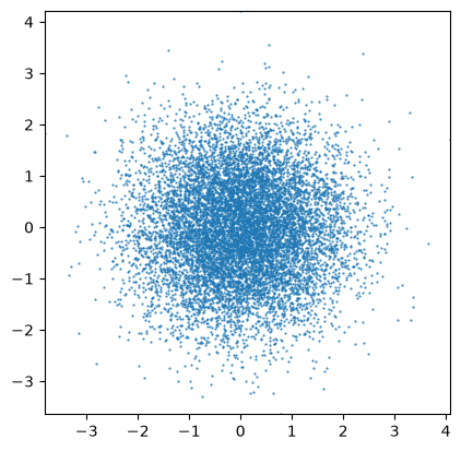
x = sc.array(dims=["row"], values=rng.normal(size=10000), unit="cm")
y = sc.array(dims=["row"], values=rng.normal(size=10000), unit="cm")
recording = sc.DataArray(
    data=sc.ones(sizes=x.sizes, unit="counts"), coords={"x": x, "y": y}
)
recording
- row: 10000
- x(row)float64cm-0.679, -0.621, ..., -0.788, 1.123
Values:
array([-0.67924997, -0.62053203, 1.33121422, ..., 0.66931119, -0.78846271, 1.12268421]) - y(row)float64cm-0.306, -0.704, ..., -0.848, 0.739
Values:
array([-0.30610691, -0.70374693, -1.00885753, ..., -0.42935023,
       -0.84826518,  0.73921398])
- (row)float64counts1.0, 1.0, ..., 1.0, 1.0
Values:
array([1., 1., 1., ..., 1., 1., 1.])
scatter(x.values, y.values)
It is very common to histogram such data.
In Scipp, histogramming has a very concise and easy-to-use syntax.
To make 8 bins in both the x and y dimensions:
image = recording.hist(y=8, x=8)
image.plot(aspect="equal")

The x and y coordinates are now bin-edge coordinates.
sc.show(image)
image
- y: 8
- x: 8
- x(x [bin-edge])float64cm-3.819, -2.831, ..., 3.095, 4.083
Values:
array([-3.81886182, -2.83110929, -1.84335675, -0.85560421, 0.13214833, 1.11990087, 2.10765341, 3.09540594, 4.08315848]) - y(y [bin-edge])float64cm-3.646, -2.663, ..., 3.236, 4.219
Values:
array([-3.64602432, -2.66291545, -1.67980659, -0.69669773,  0.28641113,
        1.26952   ,  2.25262886,  3.23573772,  4.21884658])
- (y, x)float64counts0.0, 2.0, ..., 1.0, 0.0
Values:
array([[0.000e+00, 2.000e+00, 8.000e+00, 1.200e+01, 1.000e+01, 5.000e+00,
        0.000e+00, 0.000e+00],
       [1.000e+00, 1.100e+01, 8.100e+01, 1.460e+02, 1.190e+02, 4.600e+01,
        6.000e+00, 1.000e+00],
       [4.000e+00, 6.200e+01, 3.290e+02, 7.620e+02, 6.310e+02, 2.370e+02,
        3.000e+01, 3.000e+00],
       [7.000e+00, 1.210e+02, 5.790e+02, 1.298e+03, 1.179e+03, 4.170e+02,
        7.000e+01, 2.000e+00],
       [5.000e+00, 8.800e+01, 4.440e+02, 1.030e+03, 8.770e+02, 3.240e+02,
        4.400e+01, 1.000e+00],
       [3.000e+00, 3.600e+01, 1.490e+02, 3.280e+02, 2.710e+02, 9.300e+01,
        1.400e+01, 2.000e+00],
       [0.000e+00, 5.000e+00, 1.900e+01, 3.500e+01, 3.600e+01, 1.100e+01,
        1.000e+00, 0.000e+00],
       [0.000e+00, 0.000e+00, 1.000e+00, 2.000e+00, 1.000e+00, 0.000e+00,
        1.000e+00, 0.000e+00]])
Numpy and Matplotlib return the bin edges and the data counts separately.
We have everything stored inside a single data structure.
You can, of course, adjust the number of bins:
recording.hist(y=100, x=100).plot(aspect="equal")

Exercise 3: Histogramming#
We found a 2D detector that reads your mood!
We recorded a signal with it, and now we can visualize the signal by histogramming.
from scipp_utils import load_signal_to_histogram

signal_rng = np.random.default_rng(1)
signal = load_signal_to_histogram(signal_rng)
signal
- row: 203700
- x(row)float64cm7.278, -16.296, ..., 0.018, 0.016
Values:
array([ 7.27805283e+00, -1.62959448e+01, -7.09559402e+00, ..., 1.89787051e-02, 1.81696472e-02, 1.60307256e-02]) - y(row)float64cm0.432, -0.784, ..., 0.061, 0.060
Values:
array([ 0.43193503, -0.78422306, -9.62131874, ...,  0.06044533,
        0.06091188,  0.05965346])
- (row)float64counts1.0, 1.0, ..., 1.0, 1.0
Values:
array([1., 1., 1., ..., 1., 1., 1.])
Exercise 3-1: Number of bins for histogramming.#
First, we need to find the right number of bins to histogram the signal.
We tried 200 bins and 4 bins for each axis, but none of them seems meaningful!
signal.hist(x=200, y=200).plot() + signal.hist(x=4, y=4).plot()

Solution:

Exercise 3-2: Custom histogram edges.#
However, there is a suspicious hot spot in the very middle of the image.
We want to investigate those signals within the specific range of x and y.
Let’s histogram the hot spot and see what is in there.
You can histogram the data with custom histogram edges like below.
Hint:
hist_edges_x = sc.linspace(dim="x", start=-10, stop=10, unit="cm", num=200)
hist_edges_y = sc.linspace(dim="y", start=-10, stop=10, unit="cm", num=200)
signal.hist(x=hist_edges_x, y=hist_edges_y).plot()
Solution:

3. Binned data#
Scipp distinguishes histogrammed data from binned data:
Histogrammed data refers to regular dense arrays of, e.g., floating-point values with an associated bin-edge coordinate.
Binned data refers to the precursor of histogrammed data, i.e., each bin contains a “list” of contributing events or values. Binned data can be converted into a histogram by computing the sum over all events or values in a bin.

This is conceptually similar to a multi-dimensional  .
.
It is best illustrated with an example of data analysis. For this, we will use one of the NYC taxi datasets.
NYC yellow taxi dataset#
(https://vaex.readthedocs.io/en/latest/datasets.html, Dataset from 2015, obtained as a HDF5 file from the Vaex docs, and subsequently cleaned of outliers).
For today, we will use a small set of it.
file = fetch_data("4-reduction/nyc_taxi_data_2015_small")
# %matplotlib widget

da = sc.io.load_hdf5(file)
da
- row: 17839810
- dropoff_datetime(row)datetime64s2014-12-16T02:28:00, 2015-01-10T20:58:31, ..., 2016-01-01T00:11:37, 2016-01-01T00:14:14
Values:
array(['2014-12-16T02:28:00', '2015-01-10T20:58:31', '2015-01-10T20:39:23', ..., '2016-01-01T00:06:43', '2016-01-01T00:11:37', '2016-01-01T00:14:14'], dtype='datetime64[s]') - dropoff_hour(row)int64𝟙2, 20, ..., 0, 0
Values:
array([ 2, 20, 20, ..., 0, 0, 0]) - dropoff_latitude(row)float64deg40.743, 40.750, ..., 40.763, 40.696
Values:
array([40.74289322, 40.74963379, 40.73989487, ..., 40.74245071, 40.76282883, 40.69619751]) - dropoff_longitude(row)float64deg-73.996, -73.992, ..., -73.925, -73.980
Values:
array([-73.99645996, -73.99246979, -73.99521637, ..., -73.97740936, -73.92475128, -73.98009491]) - fare_amount(row)float64\$5.0, 14.0, ..., 12.5, 17.0
Values:
array([ 5. , 14. , 6. , ..., 10.5, 12.5, 17. ]) - pickup_datetime(row)datetime64s2014-12-16T02:26:00, 2015-01-10T20:33:39, ..., 2015-12-31T23:59:48, 2015-12-31T23:59:55
Values:
array(['2014-12-16T02:26:00', '2015-01-10T20:33:39', '2015-01-10T20:33:41', ..., '2015-12-31T23:59:46', '2015-12-31T23:59:48', '2015-12-31T23:59:55'], dtype='datetime64[s]') - pickup_hour(row)int64𝟙2, 20, ..., 23, 23
Values:
array([ 2, 20, 20, ..., 23, 23, 23]) - pickup_latitude(row)float64deg40.756, 40.726, ..., 40.764, 40.731
Values:
array([40.75642014, 40.72600937, 40.73177719, ..., 40.77241898, 40.7635498 , 40.73109055]) - pickup_longitude(row)float64deg-73.987, -73.983, ..., -73.971, -73.982
Values:
array([-73.98672485, -73.98327637, -74.0067215 , ..., -73.9466095 , -73.97135925, -73.98199463]) - tip_amount(row)float64\$0.0, 0.0, ..., 0.0, 0.0
Values:
array([0., 0., 0., ..., 0., 0., 0.]) - trip_distance(row)float64mi1.090, 2.200, ..., 3.130, 5.070
Values:
array([1.09000003, 2.20000005, 1.10000002, ..., 2.79999995, 3.13000011,
       5.07000017])
- (row)float64counts1.0, 1.0, ..., 1.0, 1.0
Values:
array([1., 1., 1., ..., 1., 1., 1.])
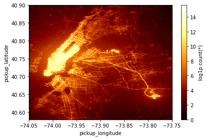
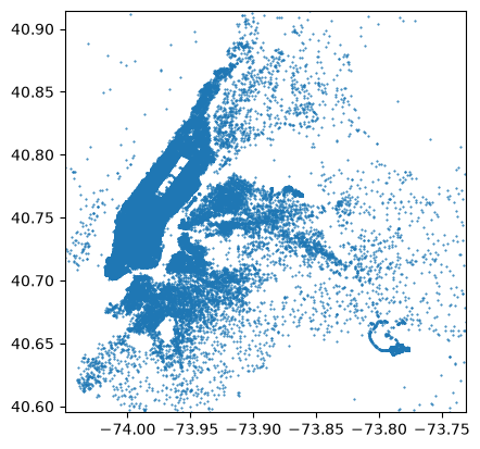
n = 100
x = da.coords["dropoff_longitude"].values[::n]
y = da.coords["dropoff_latitude"].values[::n]
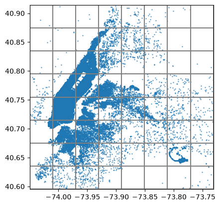
scatter(x, y)
Binning the data records#
Working with binned data is most efficient when keeping the number of bins relatively low.
Binning is essentially like overlaying a grid of bin edges onto our data
ax = scatter(x, y, get_ax=True)
for lon in np.linspace(*ax.get_xlim(), 9):
    ax.axvline(lon, color="gray")
for lat in np.linspace(*ax.get_ylim(), 9):
    ax.axhline(lat, color="gray")
# Bin into 8 longitude & latitude bins
binned = da.bin(dropoff_latitude=8, dropoff_longitude=8)
binned
- dropoff_latitude: 8
- dropoff_longitude: 8
- dropoff_latitude(dropoff_latitude [bin-edge])float64deg40.595, 40.635, ..., 40.875, 40.915
Values:
array([40.59500122, 40.63499641, 40.67499161, 40.7149868 , 40.75498199, 40.79497719, 40.83497238, 40.87496758, 40.91496277]) - dropoff_longitude(dropoff_longitude [bin-edge])float64deg-74.050, -74.010, ..., -73.770, -73.730
Values:
array([-74.04999542, -74.00999641, -73.96999741, -73.9299984 ,
       -73.88999939, -73.85000038, -73.81000137, -73.77000237,
       -73.73000336])
- (dropoff_latitude, dropoff_longitude)float64countsbinned data [len=16129, len=12695, ..., len=500, len=12]
dim='row',
content=DataArray(
          dims=(row: 17839810),
          data=float64[counts],
          coords={'dropoff_datetime':datetime64[s], 'pickup_datetime':datetime64[s],
                  'fare_amount':float64[\$], 'trip_distance':float64[mi],
                  'tip_amount':float64[\$], 'dropoff_latitude':float64[deg],
                  'dropoff_longitude':float64[deg], 'pickup_latitude':float64[deg],
                  'pickup_longitude':float64[deg], 'dropoff_hour':int64[dimensionless],
                  'pickup_hour':int64[dimensionless]})
# Histogramming is summing all the counts in each bin
binned_sum = binned.bins.sum()

binned_sum.plot(aspect="equal", norm="log")

Selecting/slicing bins#
Binning groups the data into bins, but keeps the underlying table of records.
No information is lost, it is simply re-ordered.
The bins can then be used for slicing the data, providing extremely efficient data selection and filtering.
manh = binned["dropoff_longitude", 1]["dropoff_latitude", 4]
manh
- dropoff_latitude(dropoff_latitude [bin-edge])float64deg40.755, 40.795
Values:
array([40.75498199, 40.79497719]) - dropoff_longitude(dropoff_longitude [bin-edge])float64deg-74.010, -73.970
Values:
array([-74.00999641, -73.96999741])
- ()float64countsbinned data [len=4215195]
dim='row',
content=DataArray(
          dims=(row: 17839810),
          data=float64[counts],
          coords={'dropoff_datetime':datetime64[s], 'pickup_datetime':datetime64[s],
                  'fare_amount':float64[\$], 'trip_distance':float64[mi],
                  'tip_amount':float64[\$], 'dropoff_latitude':float64[deg],
                  'dropoff_longitude':float64[deg], 'pickup_latitude':float64[deg],
                  'pickup_longitude':float64[deg], 'dropoff_hour':int64[dimensionless],
                  'pickup_hour':int64[dimensionless]})
# We can now histogram this with a much finer resolution

manh.hist(dropoff_latitude=300, dropoff_longitude=300).plot(norm="log", aspect="equal")

# We select another bin, which contains the JFK airport

jfk = binned["dropoff_longitude", 6]["dropoff_latitude", 1]
jfk.hist(dropoff_latitude=300, dropoff_longitude=300).plot(norm="log", aspect="equal")

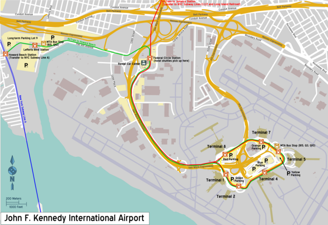
(https://commons.wikimedia.org/wiki/File:JFK_airport_terminal_map.png)
Binning into a new dimension#
Data that has already been binned can also be binned further into new dimensions.
manh
- dropoff_latitude(dropoff_latitude [bin-edge])float64deg40.755, 40.795
Values:
array([40.75498199, 40.79497719]) - dropoff_longitude(dropoff_longitude [bin-edge])float64deg-74.010, -73.970
Values:
array([-74.00999641, -73.96999741])
- ()float64countsbinned data [len=4215195]
dim='row',
content=DataArray(
          dims=(row: 17839810),
          data=float64[counts],
          coords={'dropoff_datetime':datetime64[s], 'pickup_datetime':datetime64[s],
                  'fare_amount':float64[\$], 'trip_distance':float64[mi],
                  'tip_amount':float64[\$], 'dropoff_latitude':float64[deg],
                  'dropoff_longitude':float64[deg], 'pickup_latitude':float64[deg],
                  'pickup_longitude':float64[deg], 'dropoff_hour':int64[dimensionless],
                  'pickup_hour':int64[dimensionless]})
We look at the trip distances inside the Manhattan and JFK bins we have selected above.
# Use 100 distance bins
manh_dist = manh.bin(trip_distance=100)
manh_dist
- trip_distance: 100
- dropoff_latitude(dropoff_latitude [bin-edge])float64deg40.755, 40.795
Values:
array([40.75498199, 40.79497719]) - dropoff_longitude(dropoff_longitude [bin-edge])float64deg-74.010, -73.970
Values:
array([-74.00999641, -73.96999741]) - trip_distance(trip_distance [bin-edge])float64mi0.020, 0.781, ..., 75.379, 76.140
Values:
array([1.99999996e-02, 7.81199993e-01, 1.54239999e+00, 2.30359998e+00,
       3.06479998e+00, 3.82599997e+00, 4.58719996e+00, 5.34839996e+00,
       6.10959995e+00, 6.87079994e+00, 7.63199994e+00, 8.39319993e+00,
       9.15439993e+00, 9.91559992e+00, 1.06767999e+01, 1.14379999e+01,
       1.21991999e+01, 1.29603999e+01, 1.37215999e+01, 1.44827999e+01,
       1.52439999e+01, 1.60051999e+01, 1.67663999e+01, 1.75275999e+01,
       1.82887999e+01, 1.90499998e+01, 1.98111998e+01, 2.05723998e+01,
       2.13335998e+01, 2.20947998e+01, 2.28559998e+01, 2.36171998e+01,
       2.43783998e+01, 2.51395998e+01, 2.59007998e+01, 2.66619998e+01,
       2.74231998e+01, 2.81843998e+01, 2.89455998e+01, 2.97067998e+01,
       3.04679998e+01, 3.12291997e+01, 3.19903997e+01, 3.27515997e+01,
       3.35127997e+01, 3.42739997e+01, 3.50351997e+01, 3.57963997e+01,
       3.65575997e+01, 3.73187997e+01, 3.80799997e+01, 3.88411997e+01,
       3.96023997e+01, 4.03635997e+01, 4.11247997e+01, 4.18859997e+01,
       4.26471997e+01, 4.34083997e+01, 4.41695996e+01, 4.49307996e+01,
       4.56919996e+01, 4.64531996e+01, 4.72143996e+01, 4.79755996e+01,
       4.87367996e+01, 4.94979996e+01, 5.02591996e+01, 5.10203996e+01,
       5.17815996e+01, 5.25427996e+01, 5.33039996e+01, 5.40651996e+01,
       5.48263996e+01, 5.55875996e+01, 5.63487995e+01, 5.71099995e+01,
       5.78711995e+01, 5.86323995e+01, 5.93935995e+01, 6.01547995e+01,
       6.09159995e+01, 6.16771995e+01, 6.24383995e+01, 6.31995995e+01,
       6.39607995e+01, 6.47219995e+01, 6.54831995e+01, 6.62443995e+01,
       6.70055995e+01, 6.77667995e+01, 6.85279995e+01, 6.92891994e+01,
       7.00503994e+01, 7.08115994e+01, 7.15727994e+01, 7.23339994e+01,
       7.30951994e+01, 7.38563994e+01, 7.46175994e+01, 7.53787994e+01,
       7.61399994e+01])
- (trip_distance)float64countsbinned data [len=676736, len=1480372, ..., len=0, len=1]
dim='row',
content=DataArray(
          dims=(row: 4215195),
          data=float64[counts],
          coords={'dropoff_datetime':datetime64[s], 'pickup_datetime':datetime64[s],
                  'fare_amount':float64[\$], 'trip_distance':float64[mi],
                  'tip_amount':float64[\$], 'dropoff_latitude':float64[deg],
                  'dropoff_longitude':float64[deg], 'pickup_latitude':float64[deg],
                  'pickup_longitude':float64[deg], 'dropoff_hour':int64[dimensionless],
                  'pickup_hour':int64[dimensionless]})
manh_dist.hist().plot()

jfk_dist = jfk.bin(trip_distance=100)
jfk_dist.hist().plot()

Other operations on bins: what is the fare amount as a function of distance?#
In addition to summing/histogramming, bins can be used for other reduction operations:
min(),max(), andmean().
manh_dist
- trip_distance: 100
- dropoff_latitude(dropoff_latitude [bin-edge])float64deg40.755, 40.795
Values:
array([40.75498199, 40.79497719]) - dropoff_longitude(dropoff_longitude [bin-edge])float64deg-74.010, -73.970
Values:
array([-74.00999641, -73.96999741]) - trip_distance(trip_distance [bin-edge])float64mi0.020, 0.781, ..., 75.379, 76.140
Values:
array([1.99999996e-02, 7.81199993e-01, 1.54239999e+00, 2.30359998e+00,
       3.06479998e+00, 3.82599997e+00, 4.58719996e+00, 5.34839996e+00,
       6.10959995e+00, 6.87079994e+00, 7.63199994e+00, 8.39319993e+00,
       9.15439993e+00, 9.91559992e+00, 1.06767999e+01, 1.14379999e+01,
       1.21991999e+01, 1.29603999e+01, 1.37215999e+01, 1.44827999e+01,
       1.52439999e+01, 1.60051999e+01, 1.67663999e+01, 1.75275999e+01,
       1.82887999e+01, 1.90499998e+01, 1.98111998e+01, 2.05723998e+01,
       2.13335998e+01, 2.20947998e+01, 2.28559998e+01, 2.36171998e+01,
       2.43783998e+01, 2.51395998e+01, 2.59007998e+01, 2.66619998e+01,
       2.74231998e+01, 2.81843998e+01, 2.89455998e+01, 2.97067998e+01,
       3.04679998e+01, 3.12291997e+01, 3.19903997e+01, 3.27515997e+01,
       3.35127997e+01, 3.42739997e+01, 3.50351997e+01, 3.57963997e+01,
       3.65575997e+01, 3.73187997e+01, 3.80799997e+01, 3.88411997e+01,
       3.96023997e+01, 4.03635997e+01, 4.11247997e+01, 4.18859997e+01,
       4.26471997e+01, 4.34083997e+01, 4.41695996e+01, 4.49307996e+01,
       4.56919996e+01, 4.64531996e+01, 4.72143996e+01, 4.79755996e+01,
       4.87367996e+01, 4.94979996e+01, 5.02591996e+01, 5.10203996e+01,
       5.17815996e+01, 5.25427996e+01, 5.33039996e+01, 5.40651996e+01,
       5.48263996e+01, 5.55875996e+01, 5.63487995e+01, 5.71099995e+01,
       5.78711995e+01, 5.86323995e+01, 5.93935995e+01, 6.01547995e+01,
       6.09159995e+01, 6.16771995e+01, 6.24383995e+01, 6.31995995e+01,
       6.39607995e+01, 6.47219995e+01, 6.54831995e+01, 6.62443995e+01,
       6.70055995e+01, 6.77667995e+01, 6.85279995e+01, 6.92891994e+01,
       7.00503994e+01, 7.08115994e+01, 7.15727994e+01, 7.23339994e+01,
       7.30951994e+01, 7.38563994e+01, 7.46175994e+01, 7.53787994e+01,
       7.61399994e+01])
- (trip_distance)float64countsbinned data [len=676736, len=1480372, ..., len=0, len=1]
dim='row',
content=DataArray(
          dims=(row: 4215195),
          data=float64[counts],
          coords={'dropoff_datetime':datetime64[s], 'pickup_datetime':datetime64[s],
                  'fare_amount':float64[\$], 'trip_distance':float64[mi],
                  'tip_amount':float64[\$], 'dropoff_latitude':float64[deg],
                  'dropoff_longitude':float64[deg], 'pickup_latitude':float64[deg],
                  'pickup_longitude':float64[deg], 'dropoff_hour':int64[dimensionless],
                  'pickup_hour':int64[dimensionless]})
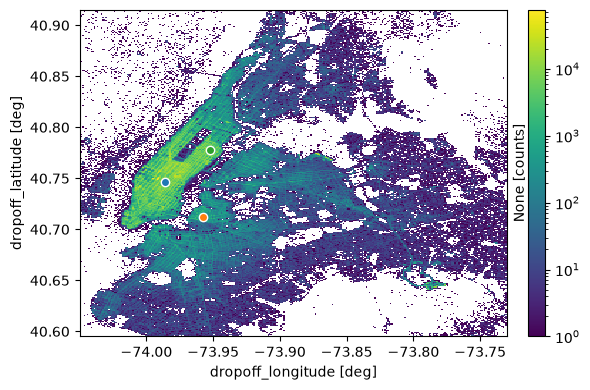
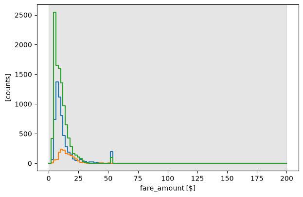
To get the minimum and maximum fares for all trips that ended inside our Manhattan area, we can do
manh_dist.bins.coords["fare_amount"].min(), manh.bins.coords["fare_amount"].max()
(<scipp.Variable> ()    float64              [$]  -80,
 <scipp.Variable> ()    float64              [$]  900)
These values are somewhat strange, indicative of bad data in the table.
We restrict our fare range from 0 to 200 dollars.
# Make 100 bins between 0 and 200 dollars
nbins = 100
fare_bins = sc.linspace("fare_amount", 0, 200, nbins + 1, unit="$")

# Bin & plot our data
manh_dist.bin(fare_amount=fare_bins).hist().transpose().plot(norm="log")

Some things we can say about the data:
there appears to be a (somewhat expected) correlation between fare amount and trip distance: the further you go, the more you’ll have to pay
for a given trip distance, clients usually pay above the diagonal line, rarely below
there appears to be a magic fare amount of $52 that will take you anywhere from 0 to 60 miles!
4. Plopp: interactive data visualization tools#
import plopp as pp

fare_lat_lon = da.hist(
    fare_amount=fare_bins, dropoff_latitude=300, dropoff_longitude=300
)
fare_lat_lon
- fare_amount: 100
- dropoff_latitude: 300
- dropoff_longitude: 300
- dropoff_latitude(dropoff_latitude [bin-edge])float64deg40.595, 40.596, ..., 40.914, 40.915
Values:
array([40.59500122, 40.59606776, 40.5971343 , 40.59820084, 40.59926737, 40.60033391, 40.60140045, 40.60246699, 40.60353353, 40.60460007, 40.60566661, 40.60673314, 40.60779968, 40.60886622, 40.60993276, 40.6109993 , 40.61206584, 40.61313238, 40.61419891, 40.61526545, 40.61633199, 40.61739853, 40.61846507, 40.61953161, 40.62059814, 40.62166468, 40.62273122, 40.62379776, 40.6248643 , 40.62593084, 40.62699738, 40.62806391, 40.62913045, 40.63019699, 40.63126353, 40.63233007, 40.63339661, 40.63446314, 40.63552968, 40.63659622, 40.63766276, 40.6387293 , 40.63979584, 40.64086238, 40.64192891, 40.64299545, 40.64406199, 40.64512853, 40.64619507, 40.64726161, 40.64832815, 40.64939468, 40.65046122, 40.65152776, 40.6525943 , 40.65366084, 40.65472738, 40.65579391, 40.65686045, 40.65792699, 40.65899353, 40.66006007, 40.66112661, 40.66219315, 40.66325968, 40.66432622, 40.66539276, 40.6664593 , 40.66752584, 40.66859238, 40.66965892, 40.67072545, 40.67179199, 40.67285853, 40.67392507, 40.67499161, 40.67605815, 40.67712468, 40.67819122, 40.67925776, 40.6803243 , 40.68139084, 40.68245738, 40.68352392, 40.68459045, 40.68565699, 40.68672353, 40.68779007, 40.68885661, 40.68992315, 40.69098969, 40.69205622, 40.69312276, 40.6941893 , 40.69525584, 40.69632238, 40.69738892, 40.69845545, 40.69952199, 40.70058853, 40.70165507, 40.70272161, 40.70378815, 40.70485469, 40.70592122, 40.70698776, 40.7080543 , 40.70912084, 40.71018738, 40.71125392, 40.71232045, 40.71338699, 40.71445353, 40.71552007, 40.71658661, 40.71765315, 40.71871969, 40.71978622, 40.72085276, 40.7219193 , 40.72298584, 40.72405238, 40.72511892, 40.72618546, 40.72725199, 40.72831853, 40.72938507, 40.73045161, 40.73151815, 40.73258469, 40.73365122, 40.73471776, 40.7357843 , 40.73685084, 40.73791738, 40.73898392, 40.74005046, 40.74111699, 40.74218353, 40.74325007, 40.74431661, 40.74538315, 40.74644969, 40.74751623, 40.74858276, 40.7496493 , 40.75071584, 40.75178238, 40.75284892, 40.75391546, 40.75498199, 40.75604853, 40.75711507, 40.75818161, 40.75924815, 40.76031469, 40.76138123, 40.76244776, 40.7635143 , 40.76458084, 40.76564738, 40.76671392, 40.76778046, 40.768847 , 40.76991353, 40.77098007, 40.77204661, 40.77311315, 40.77417969, 40.77524623, 40.77631276, 40.7773793 , 40.77844584, 40.77951238, 40.78057892, 40.78164546, 40.782712 , 40.78377853, 40.78484507, 40.78591161, 40.78697815, 40.78804469, 40.78911123, 40.79017776, 40.7912443 , 40.79231084, 40.79337738, 40.79444392, 40.79551046, 40.796577 , 40.79764353, 40.79871007, 40.79977661, 40.80084315, 40.80190969, 40.80297623, 40.80404277, 40.8051093 , 40.80617584, 40.80724238, 40.80830892, 40.80937546, 40.810442 , 40.81150853, 40.81257507, 40.81364161, 40.81470815, 40.81577469, 40.81684123, 40.81790777, 40.8189743 , 40.82004084, 40.82110738, 40.82217392, 40.82324046, 40.824307 , 40.82537354, 40.82644007, 40.82750661, 40.82857315, 40.82963969, 40.83070623, 40.83177277, 40.8328393 , 40.83390584, 40.83497238, 40.83603892, 40.83710546, 40.838172 , 40.83923854, 40.84030507, 40.84137161, 40.84243815, 40.84350469, 40.84457123, 40.84563777, 40.84670431, 40.84777084, 40.84883738, 40.84990392, 40.85097046, 40.852037 , 40.85310354, 40.85417007, 40.85523661, 40.85630315, 40.85736969, 40.85843623, 40.85950277, 40.86056931, 40.86163584, 40.86270238, 40.86376892, 40.86483546, 40.865902 , 40.86696854, 40.86803507, 40.86910161, 40.87016815, 40.87123469, 40.87230123, 40.87336777, 40.87443431, 40.87550084, 40.87656738, 40.87763392, 40.87870046, 40.879767 , 40.88083354, 40.88190008, 40.88296661, 40.88403315, 40.88509969, 40.88616623, 40.88723277, 40.88829931, 40.88936584, 40.89043238, 40.89149892, 40.89256546, 40.893632 , 40.89469854, 40.89576508, 40.89683161, 40.89789815, 40.89896469, 40.90003123, 40.90109777, 40.90216431, 40.90323085, 40.90429738, 40.90536392, 40.90643046, 40.907497 , 40.90856354, 40.90963008, 40.91069661, 40.91176315, 40.91282969, 40.91389623, 40.91496277]) - dropoff_longitude(dropoff_longitude [bin-edge])float64deg-74.050, -74.049, ..., -73.731, -73.730
Values:
array([-74.04999542, -74.04892878, -74.04786214, -74.0467955 , -74.04572886, -74.04466222, -74.04359558, -74.04252894, -74.0414623 , -74.04039566, -74.03932902, -74.03826238, -74.03719574, -74.0361291 , -74.03506246, -74.03399582, -74.03292918, -74.03186254, -74.0307959 , -74.02972926, -74.02866262, -74.02759598, -74.02652934, -74.0254627 , -74.02439606, -74.02332942, -74.02226278, -74.02119614, -74.0201295 , -74.01906286, -74.01799622, -74.01692958, -74.01586294, -74.0147963 , -74.01372965, -74.01266301, -74.01159637, -74.01052973, -74.00946309, -74.00839645, -74.00732981, -74.00626317, -74.00519653, -74.00412989, -74.00306325, -74.00199661, -74.00092997, -73.99986333, -73.99879669, -73.99773005, -73.99666341, -73.99559677, -73.99453013, -73.99346349, -73.99239685, -73.99133021, -73.99026357, -73.98919693, -73.98813029, -73.98706365, -73.98599701, -73.98493037, -73.98386373, -73.98279709, -73.98173045, -73.98066381, -73.97959717, -73.97853053, -73.97746389, -73.97639725, -73.97533061, -73.97426397, -73.97319733, -73.97213069, -73.97106405, -73.96999741, -73.96893077, -73.96786413, -73.96679749, -73.96573085, -73.9646642 , -73.96359756, -73.96253092, -73.96146428, -73.96039764, -73.959331 , -73.95826436, -73.95719772, -73.95613108, -73.95506444, -73.9539978 , -73.95293116, -73.95186452, -73.95079788, -73.94973124, -73.9486646 , -73.94759796, -73.94653132, -73.94546468, -73.94439804, -73.9433314 , -73.94226476, -73.94119812, -73.94013148, -73.93906484, -73.9379982 , -73.93693156, -73.93586492, -73.93479828, -73.93373164, -73.932665 , -73.93159836, -73.93053172, -73.92946508, -73.92839844, -73.9273318 , -73.92626516, -73.92519852, -73.92413188, -73.92306524, -73.9219986 , -73.92093196, -73.91986532, -73.91879868, -73.91773204, -73.9166654 , -73.91559875, -73.91453211, -73.91346547, -73.91239883, -73.91133219, -73.91026555, -73.90919891, -73.90813227, -73.90706563, -73.90599899, -73.90493235, -73.90386571, -73.90279907, -73.90173243, -73.90066579, -73.89959915, -73.89853251, -73.89746587, -73.89639923, -73.89533259, -73.89426595, -73.89319931, -73.89213267, -73.89106603, -73.88999939, -73.88893275, -73.88786611, -73.88679947, -73.88573283, -73.88466619, -73.88359955, -73.88253291, -73.88146627, -73.88039963, -73.87933299, -73.87826635, -73.87719971, -73.87613307, -73.87506643, -73.87399979, -73.87293315, -73.87186651, -73.87079987, -73.86973323, -73.86866659, -73.86759995, -73.8665333 , -73.86546666, -73.86440002, -73.86333338, -73.86226674, -73.8612001 , -73.86013346, -73.85906682, -73.85800018, -73.85693354, -73.8558669 , -73.85480026, -73.85373362, -73.85266698, -73.85160034, -73.8505337 , -73.84946706, -73.84840042, -73.84733378, -73.84626714, -73.8452005 , -73.84413386, -73.84306722, -73.84200058, -73.84093394, -73.8398673 , -73.83880066, -73.83773402, -73.83666738, -73.83560074, -73.8345341 , -73.83346746, -73.83240082, -73.83133418, -73.83026754, -73.8292009 , -73.82813426, -73.82706762, -73.82600098, -73.82493434, -73.8238677 , -73.82280106, -73.82173442, -73.82066778, -73.81960114, -73.8185345 , -73.81746785, -73.81640121, -73.81533457, -73.81426793, -73.81320129, -73.81213465, -73.81106801, -73.81000137, -73.80893473, -73.80786809, -73.80680145, -73.80573481, -73.80466817, -73.80360153, -73.80253489, -73.80146825, -73.80040161, -73.79933497, -73.79826833, -73.79720169, -73.79613505, -73.79506841, -73.79400177, -73.79293513, -73.79186849, -73.79080185, -73.78973521, -73.78866857, -73.78760193, -73.78653529, -73.78546865, -73.78440201, -73.78333537, -73.78226873, -73.78120209, -73.78013545, -73.77906881, -73.77800217, -73.77693553, -73.77586889, -73.77480225, -73.77373561, -73.77266897, -73.77160233, -73.77053569, -73.76946905, -73.7684024 , -73.76733576, -73.76626912, -73.76520248, -73.76413584, -73.7630692 , -73.76200256, -73.76093592, -73.75986928, -73.75880264, -73.757736 , -73.75666936, -73.75560272, -73.75453608, -73.75346944, -73.7524028 , -73.75133616, -73.75026952, -73.74920288, -73.74813624, -73.7470696 , -73.74600296, -73.74493632, -73.74386968, -73.74280304, -73.7417364 , -73.74066976, -73.73960312, -73.73853648, -73.73746984, -73.7364032 , -73.73533656, -73.73426992, -73.73320328, -73.73213664, -73.73107 , -73.73000336]) - fare_amount(fare_amount [bin-edge])float64\$0.0, 2.0, ..., 198.0, 200.0
Values:
array([  0.,   2.,   4.,   6.,   8.,  10.,  12.,  14.,  16.,  18.,  20.,
        22.,  24.,  26.,  28.,  30.,  32.,  34.,  36.,  38.,  40.,  42.,
        44.,  46.,  48.,  50.,  52.,  54.,  56.,  58.,  60.,  62.,  64.,
        66.,  68.,  70.,  72.,  74.,  76.,  78.,  80.,  82.,  84.,  86.,
        88.,  90.,  92.,  94.,  96.,  98., 100., 102., 104., 106., 108.,
       110., 112., 114., 116., 118., 120., 122., 124., 126., 128., 130.,
       132., 134., 136., 138., 140., 142., 144., 146., 148., 150., 152.,
       154., 156., 158., 160., 162., 164., 166., 168., 170., 172., 174.,
       176., 178., 180., 182., 184., 186., 188., 190., 192., 194., 196.,
       198., 200.])
- (fare_amount, dropoff_latitude, dropoff_longitude)float64counts0.0, 0.0, ..., 0.0, 0.0
Values:
array([[[0., 0., 0., ..., 0., 0., 0.],
        [0., 0., 0., ..., 0., 0., 0.],
        [0., 0., 0., ..., 0., 0., 0.],
        ...,
        [0., 0., 0., ..., 0., 0., 0.],
        [0., 0., 0., ..., 0., 0., 0.],
        [0., 0., 0., ..., 0., 0., 0.]],

       [[0., 0., 0., ..., 0., 0., 0.],
        [0., 0., 0., ..., 0., 0., 0.],
        [0., 0., 0., ..., 0., 0., 0.],
        ...,
        [0., 0., 0., ..., 0., 0., 0.],
        [0., 0., 0., ..., 0., 0., 0.],
        [0., 0., 0., ..., 0., 0., 0.]],

       [[0., 0., 0., ..., 0., 0., 0.],
        [0., 0., 0., ..., 0., 0., 0.],
        [0., 0., 0., ..., 0., 0., 0.],
        ...,
        [0., 0., 0., ..., 0., 0., 0.],
        [0., 0., 0., ..., 0., 0., 0.],
        [0., 0., 0., ..., 0., 0., 0.]],

       ...,

       [[0., 0., 0., ..., 0., 0., 0.],
        [0., 0., 0., ..., 0., 0., 0.],
        [0., 0., 0., ..., 0., 0., 0.],
        ...,
        [0., 0., 0., ..., 0., 0., 0.],
        [0., 0., 0., ..., 0., 0., 0.],
        [0., 0., 0., ..., 0., 0., 0.]],

       [[0., 0., 0., ..., 0., 0., 0.],
        [0., 0., 0., ..., 0., 0., 0.],
        [0., 0., 0., ..., 0., 0., 0.],
        ...,
        [0., 0., 0., ..., 0., 0., 0.],
        [0., 0., 0., ..., 0., 0., 0.],
        [0., 0., 0., ..., 0., 0., 0.]],

       [[0., 0., 0., ..., 0., 0., 0.],
        [0., 0., 0., ..., 0., 0., 0.],
        [0., 0., 0., ..., 0., 0., 0.],
        ...,
        [0., 0., 0., ..., 0., 0., 0.],
        [0., 0., 0., ..., 0., 0., 0.],
        [0., 0., 0., ..., 0., 0., 0.]]])
%matplotlib widget

inspect = pp.inspector(fare_lat_lon, dim="fare_amount", norm="log")
inspect
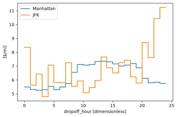
Exercise 4.1: Rush hours#
Histogram the Manhattan and JFK bins according to hour-of-the-day, to show the quiet and busy hours for both boroughs.
Solution:
Exercise 4.2: Expensive hours#
The final exercise is to create an interactive figure that will show histograms of how expensive trips were, as a function of the hour-of-the-day, for the entire dataset.
You should:
Create a
price_per_milecoordinate on the original datasetdaBin
dausing two dimensions: hour-of-the-day andprice_per_mileUse Plopp’s
superplotfunction to make a figure with a 1D histogram and an interactive slider to navigate the hour dimension
Use the slider to find the hour of the day when trips are the most expensive!
Hint: For binning in hour-of-the-day, using 24 bins should work well.
For binning in price_per_mile, you will have to manually set the bin boundaries.
Solution:
Bonus Exercise#
You decided to join an exchange program in NY.
But living expenses are too high there, even compared to Copenhagen!
Luckily, you can take over a car from a previous student in the same program, and you are allowed to have a part-time job for 2 hours every day, and there is no limit of income.
So you decide to be a shared-car driver. Your goal is to maximize your income within those 2 hours, so you are going to analyse which hours to drive in which borough!
You are free to choose 2 hours among all 24 in a day, and there are 2 places, Manhattan and JFK airport, where you can be registered as a driver.
Solution