Simulation#
At the ESS we have used simulations extensively to design and optimize the facility.
Monte Carlo Ray-tracing#
For simulation of neutron scattering the most popular technique is Monte Carlo ray-tracing. Lets look at the two separately and then merge them.
Monte Carlo#
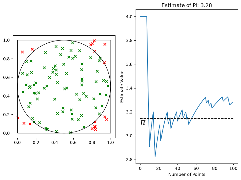
The Monte Carlo technique relies on using random numbers to estimate values that would otherwise be difficult to calculate. It is a computationally expensive technique, but is very versatile and often work when other more efficient techniques fail. For example one could estimate the value of \(\pi\) by using random sampling to find the ratio of the areas of a circle and a square as shown below. The ratio of their area’s can simply be estimated by the number of random points falling outside and inside the circle, from which an estimate of \(\pi\) can be calculated. The more random points we use, the better an estimate of \(\pi\).
import monte_carlo
monte_carlo.example()
Ray-tracing#
The ray-tracing part of the simulation deals with the paths of the neutrons through space. Thus the geometric effects in the optics can be understood, as the path of the neutrons are traced through the known guide system.
Monte Carlo ray-tracing#
Combining these techniques one can start the rays with random velocities drawn from a distribution that resembles the real source, trace the path of the neutrons through the instrument, and at each interaction, random numbers will be used to sample the behavior using the known probability distributions. Repeating this with many rays allow us to estimate for example the flux at the detector, or even the distribution of flux on the detector.
McStas#
The McStas software package is a framework for fast Monte Carlo ray-tracing simulations of neutron scattering instruments. The main feature of the code is that it effectively connects a number of smaller pieces of codes called components that each describe a spatially separated part of the instrument. Examples of such components could be guide pieces, choppers, samples, monitors and so forth. Instruments are then built from a sequence of such components. When someone has an idea for something new they would like to simulate, it’s often easier to create that thing as a McStas component than it would be to write a specialized software package for the purpose. Because of this, the package grows with community contributed components.
Programming language#
The McStas core and components are all written using the C programming language, though the user interface for assembling the instrument is a meta-language built upon C. This means C code is allowed in parts the file, but it also has a section for adding these components with their parameters and physical positions / rotations with a simple syntax. There also exists a McStas python API called McStasScript, this is what will be used during this course.
Coordinate system#
To use McStas effectively it is important to understand the coordinate system. The beam direction is generally along the z direction, y points upwards against gravity and x to the left when looking in the beam direction. Furthermore each component will have its own coordinate system, and components can be placed relative to one another. The McStas core handles this complexity so each component can work in a simple local coordinate system.
Units#
McStas generally uses SI units with the exception of Å and meV and in few cases \(\mu\)s. Physical distances when placing components are given in meters and rotations in degrees. The contributed nature of components however means that their parameters could in principle have any unit, so look in their documentation to be sure, it is typically in the top of the component file.
Simulation#
Often the simulation will run to estimate a intensity, meaning neutrons per second, and will give this result with an error. This error can be reduced by using more rays for the simulation, corresponding to more Monte Carlo samples. To get the expected count from an experiment, one would have to multiply the intensity with the experiment time. It is also important to understand that the error reported by McStas has nothing to do with the expected error in an experiment, that would be calculated from the square root of the number of counts, the McStas error instead measures the quality of the intensity estimate.
Quick tutorial#
Thorough Python McStas tutorials can be found with the documentation for McStasScript here, and for examples in the C syntax one can look in the McStas package or on the package website.
Import the package#
First the package needs to be installed, then it can be imported. McStasScript also needs to be configured to access the local McStas installation, this is covered in the documentation. It is common to define a shorter name when importing to save some keystrokes, here ms is chosen.
import mcstasscript as ms
The main class is called McStas_instr, which makes an instrument object. It just needs a name, which will correspond to the name of the instrument file.
instrument = ms.McStas_instr("python_tutorial")
As we learned the instrument is composed of components. The instrument object already knows what components are available, so we can ask it to share that information:
instrument.available_components()
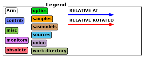
Here are the available component categories:
 contrib
 misc
 monitors
 obsolete
 optics
 samples
 sasmodels
 sources
 union
Call available_components(category_name) to display
These are categories, lets see what sources are available.
instrument.available_components("sources")
Here are all components in the sources category.
 Adapt_check     Monitor_Optimizer   Source_adapt       Source_simple
 ESS_butterfly   Source_4PI          Source_div
 ESS_moderator   Source_Maxwell_3    Source_div_quasi
 Moderator       Source_Optimizer    Source_gen
We start our instrument with a Source_div component, lets get some help on that.
instrument.component_help("Source_div")
 ___ Help Source_div ________________________________________________________________
|optional parameter|required parameter|default value|user specified value|
xwidth [m] // Width of source
yheight [m] // Height of source
focus_aw [deg] // FWHM (Gaussian) or maximal (uniform) horz. width divergence
focus_ah [deg] // FWHM (Gaussian) or maximal (uniform) vert. height divergence
E0 = 0.0 [meV] // Mean energy of neutrons.
dE = 0.0 [meV] // Energy half spread of neutrons.
lambda0 = 0.0 [Ang] // Mean wavelength of neutrons (only relevant for E0=0)
dlambda = 0.0 [Ang] // Wavelength half spread of neutrons.
gauss = 0.0 [0|1] // Criterion
flux = 1.0 [1/(s cm 2 st energy_unit)] // flux per energy unit, Angs or meV
-------------------------------------------------------------------------------------
Now we are ready to add this to our instrument. We use add_component to add the new component to our instrument, and show_components to see the current state of the instrument component sequence.
src = instrument.add_component("source", "Source_div")
instrument.show_components()
source Source_div AT (0, 0, 0) ABSOLUTE
We saved a reference to the component in the python variable src, we can print that to see more.
print(src)
COMPONENT source = Source_div(
  xwidth : Required parameter not yet specified
  yheight : Required parameter not yet specified
  focus_aw : Required parameter not yet specified
  focus_ah : Required parameter not yet specified
)
AT (0, 0, 0) ABSOLUTE
There are some required parameters for this component, lets set these to reasonable values.
src.set_parameters(xwidth=0.1, yheight=0.05,
                   focus_aw=1.2, focus_ah=2.3)
print(src)
COMPONENT source = Source_div(
  xwidth = 0.1, // [m]
  yheight = 0.05, // [m]
  focus_aw = 1.2, // [deg]
  focus_ah = 2.3 // [deg]
)
AT (0, 0, 0) ABSOLUTE
There are more optional parameters, to see them all including short explanations, one can call show_parameters on an instrument object.
src.show_parameters()
 ___ Help Source_div ________________________________________________________________
|optional parameter|required parameter|default value|user specified value|
xwidth = 0.1 [m] // Width of source
yheight = 0.05 [m] // Height of source
focus_aw = 1.2 [deg] // FWHM (Gaussian) or maximal (uniform) horz. width
                        divergence
focus_ah = 2.3 [deg] // FWHM (Gaussian) or maximal (uniform) vert. height
                        divergence
E0 = 0.0 [meV] // Mean energy of neutrons.
dE = 0.0 [meV] // Energy half spread of neutrons.
lambda0 = 0.0 [Ang] // Mean wavelength of neutrons (only relevant for E0=0)
dlambda = 0.0 [Ang] // Wavelength half spread of neutrons.
gauss = 0.0 [0|1] // Criterion
flux = 1.0 [1/(s cm 2 st energy_unit)] // flux per energy unit, Angs or meV
-------------------------------------------------------------------------------------
It seems there are two ways to define the energy range of the emitted neutrons, through energy and wavelength. Here lets use wavelength, and lets allow the wavelength to be user specified by defining a couple of instrument parameters.
wavelength_par = instrument.add_parameter("wavelength", value=5.0,
                                      comment="Wavelength in [Ang]")

wavelength_spread_par = instrument.add_parameter("wavelength_spread", value=1.2,
                                      comment="Wavelength spread in [Ang]")
We can assign these to component parameters in two ways as shown below. Either using the parameter object, or by providing the parameter name as a string.
src.set_parameters(lambda0=wavelength_par, dlambda="wavelength_spread")
print(src)
COMPONENT source = Source_div(
  xwidth = 0.1, // [m]
  yheight = 0.05, // [m]
  focus_aw = 1.2, // [deg]
  focus_ah = 2.3, // [deg]
  lambda0 = wavelength, // [Ang]
  dlambda = wavelength_spread // [Ang]
)
AT (0, 0, 0) ABSOLUTE
Now the next component we want to add is a piece of guide. We will use the component Guide_gravity, and place it in space using the set_AT method. This takes the relative position, and then a name of the coordinate system to use, which correspond to a previous component, here the source. In McStas the convention is that guide components have their opening in the center of the specified location, while for example samples are centered on that location.
guide_A = instrument.add_component("guide_A", "Guide_gravity")
guide_A.set_parameters(w1=0.05, h1=0.05, l=5, m=2.5)
guide_A.set_AT([0, 0, 2], RELATIVE="source")
We can add an additional piece of guide. Notice how we use the length of guide_A to place the start of the next guide. We can also use the component object to set the reference instead of a string.
guide_B = instrument.add_component("guide_B", "Guide_gravity")
guide_B.set_parameters(w1=0.05, h1=0.05, l=5, m=2.5)
guide_B.set_AT([0, 0, guide_A.l + 0.2], RELATIVE=guide_A)
After the guide we will place a monitor which record the spatial distribution of the beam. Notice that specifying a literal string requires double use quotation marks in McStasScript, otherwise it would be interpreted as a variable. For C it is also important that the string in the file has the “ character, so that has to be the innermost one.
mon = instrument.add_component("monitor", "PSD_monitor")
mon.set_parameters(nx=100, ny=100, filename='"PSD.dat"',
                   xwidth=0.05, yheight=0.05, restore_neutron=1)
mon.set_AT([0, 0, guide_B.l + 0.5], RELATIVE=guide_B)
Lets see the status of the components in our instrument object now.
instrument.show_components()
source  Source_div    AT (0, 0, 0)   ABSOLUTE
guide_A Guide_gravity AT (0, 0, 2)   RELATIVE source
guide_B Guide_gravity AT (0, 0, 5.2) RELATIVE guide_A
monitor PSD_monitor   AT (0, 0, 5.5) RELATIVE guide_B
If we wanted to add a monitor between guide_A and guide_B, we could place it between them in the code and rerun our notebook. This is not always possible, for example when you get a instrument object from a function call, so it’s also possible to give a keyword argument to the add_component call to place a component some other place in the sequence. Below we place a monitor after guide_A.
mon = instrument.add_component("monitor_in_guide", "PSD_monitor", after="guide_A")
mon.set_parameters(nx=100, ny=100, filename='"PSD_in_guide.dat"',
                   xwidth=0.05, yheight=0.05, restore_neutron=1)
mon.set_AT([0, 0, guide_A.l + 0.1], RELATIVE=guide_A)
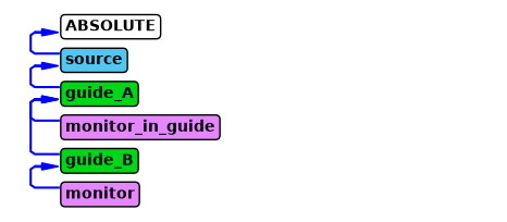
There are two tools to show the component sequence, the other is reached with the show_diagram method as below. It also shows what coordinate system each component is using, here we see both the middle monitor and guide_B are in the guide_A coordinate system.
instrument.show_diagram()
Now we would like to execute the simulation, though lets first take a look at the included parameters of the instrument, this is done with show_parameters.
instrument.show_parameters()
 wavelength         = 5.0  // Wavelength in [Ang]
 wavelength_spread  = 1.2  // Wavelength spread in [Ang]
These can be modified with set_parameters on the instrument object.
instrument.set_parameters(wavelength=2.8)
And we an see how that modified the value by calling show_parameters again
instrument.show_parameters()
 wavelength         = 2.8  // Wavelength in [Ang]
 wavelength_spread  = 1.2  // Wavelength spread in [Ang]
There are also some computational settings that can be adjusted with the settings method, here we set the number of rays and the name of the folder for the generated data. The current settings can be seen with show_settings.
instrument.settings(ncount=5E6, output_path="mcstas_data_set")
instrument.show_settings()
Instrument settings:
  ncount:           5.00e+06
  output_path:      mcstas_data_set
  run_path:         .
  package_path:     /home/runner/work/dmsc-school/dmsc-school/.pixi/envs/default/share/mcstas/resources
  executable_path:  /home/runner/work/dmsc-school/dmsc-school/.pixi/envs/default/bin
  executable:       mcrun
  force_compile:    True
  NeXus:            False
  save_comp_pars:   False
Now we are ready to execute the simulation, this is done with the backengine method. It will return a data object, so store that in a python variable, here with the name data.
data = instrument.backengine()
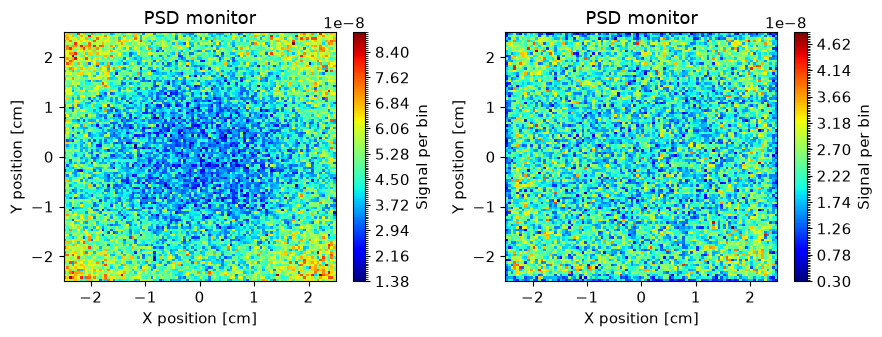
McStasScript includes functions for plotting the data, for example make_sub_plot.
ms.make_sub_plot(data)
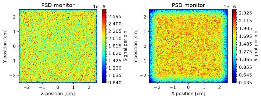
We see that there is little difference between the beam in the middle of this straight guide and after, though of course the intensities are slightly lower at the end. We can rerun the simulation at a different wavelength. Shorter wavelengths are more challenging for the guide system, so we will try that.
instrument.set_parameters(wavelength=0.8, wavelength_spread=0.1)
data = instrument.backengine()
ms.make_sub_plot(data)
Here we see a significant difference as the early reflections can be seen only in the corners. This is because the middle monitor is so close to the start of the guide that rays that would end in the center through a reflection has too steep an angle of incidence on the mirrors, and are thus not reflected.