Markov chain Monte Carlo

A popular tool in Bayesian modelling is Markov chain Monte Carlo (MCMC). This is a sampling technique that makes use of a Markov chain to sample a given probability distribution. In the context of Bayesian modelling, the probability distribution that is sampled is the posterior distribution, \(P(A|B)\), which is given by Bayes’ theorem:

(6)\[ P(A|B) = \frac{P(B|A)P(A)}{P(B)} \propto P(B|A)P(A), \]

where \(P(B|A)\) is the likelihood that we met previously, \(P(A)\) is the probability distribution that describes our prior knowledge, and \(P(B)\) is the evidence term, which in the context of MCMC is ignored as the data is not variable with the parameters \(A\).

easyCore can be combined with the MCMC library emcee to perform MCMC sampling. Before starting to sample, it is necessary to have a good estimate of the maximum likelihood (or maximum a posteriori) for the parameters, to be used as a starting point for the analysis. Below, the fitting analysis from earlier is shown for the quadratic function.

from easyCore import np
from easyCore.Objects.Variable import Parameter
from easyCore.Objects.ObjectClasses import BaseObj
from easyCore.Fitting.Fitting import Fitter

np.random.seed(123)

a_true = -0.9594
b_true = 7.294
c_true = 3.102

N = 25
x = np.linspace(0, 10, N)
yerr = 1 + 1 * np.random.rand(N)
y = a_true * x ** 2 + b_true * x + c_true
y += np.abs(y) * 0.1 * np.random.randn(N)

a = Parameter(name='a', value=a_true, fixed=False, min=-5.0, max=0.5)
b = Parameter(name='b', value=b_true, fixed=False, min=0, max=10)
c = Parameter(name='c', value=c_true, fixed=False, min=-20, max=50)

def math_model(x: np.ndarray) -> np.ndarray:
    """
    Mathematical model for a quadratic. 
    
    :x: values to calculate the model over. 
    
    :return: model values.
    """
    return a.raw_value * x ** 2 + b.raw_value * x + c.raw_value

quad = BaseObj(name='quad', a=a, b=b, c=c)
f = Fitter(quad, math_model)

res = f.fit(x=x, y=y, weights=1/yerr)

a, b, c

(<Parameter 'a': -0.95+/-0.04, bounds=[-5.0:0.5]>,
 <Parameter 'b': 7.3+/-0.4, bounds=[0:10]>,
 <Parameter 'c': 2.0+/-0.8, bounds=[-20:50]>)

To allow the calculation of the likelihood, a multidimensional normal distribution (MVN) that describes the data is constructed, where the mean is the y values and the covariance matrix is a matrix where the diagonal is the variances.

from scipy.stats import multivariate_normal

mv = multivariate_normal(mean=y, cov=np.diag(yerr ** 2))

This MVN is then used to define a function for the log-likelihood (the logarithm is often used for numerical stability).

def log_likelihood(theta: np.ndarray, x: np.ndarray) -> float:
    """
    The log-likelihood function for the data given a model. 

    :theta: the model parameters.
    :x: the value over which the model is computed.

    :return: log-likelihood for the given parameters.
    """
    a.value, b.value, c.value = theta
    model = f.evaluate(x)
    logl = mv.logpdf(model)
    return logl

The distribution that describes our prior knowledge is the prior probability, which as discussed previously consists of uniform distributions. The log-prior probability is defined with the following function.

from scipy.stats import uniform

priors = []
for p in f.fit_object.get_parameters():
    priors.append(uniform(loc=p.min, scale=p.max - p.min))

def log_prior(theta: np.ndarray) -> float:
    """
    The log-prior function for the parameters.
    
    :theta: the model parameters.

    :return: log-prior for the given parameters.
    """
    return sum([p.logpdf(theta[i]) for i, p in enumerate(priors)])

The two functions then come together to give the log-posterior function, which is the object that will be sampled.

def log_posterior(theta, x):
    return log_prior(theta) + log_likelihood(theta, x)

The emcee package can then be used to perform the MCMC sampling. Below, we perform 32 individual walks that each sample the distribution 500 times. Note that we set progress to False for the benefit of the web rendering, it might be valuable to have this as True in your Notebook.

import emcee

pos = list(res.p.values()) + 1e-4 * np.random.randn(32, 3)
nwalkers, ndim = pos.shape

nsamples = 500

sampler = emcee.EnsembleSampler(nwalkers, ndim, log_posterior, args=[x])
sampler.run_mcmc(pos, nsamples, progress=False);

The Markov chains that were investigated by the walkers in the sampling processed can be visualised as shown below.

import matplotlib.pyplot as plt

fig, axes = plt.subplots(3, figsize=(10, 4), sharex=True)
samples = sampler.get_chain()
labels = ["a", "b", "c"]
for i in range(ndim):
    ax = axes[i]
    ax.plot(samples[:, :, i], "k", alpha=0.3)
    ax.set_xlim(0, len(samples))
    ax.set_ylabel(labels[i])
    ax.yaxis.set_label_coords(-0.1, 0.5)

axes[-1].set_xlabel("step number");

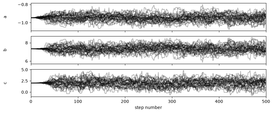
It is clear from the above plot that there is a lag period before the sampling is being carried out evenly. This means that the samples before the first (approximately) 100 steps should be ignored as they are not yet sampling evenly. We can get flat, i.e., all the walkers combined, sets of samples with the first 100 steps removed using the method below. Additionally, we perform thinning so that only every 10th sample is used (this is to remove any correlation between samples).

flat_samples = sampler.get_chain(discard=100, thin=10, flat=True)

With the flat samples, we can now plot these as histograms, using the corner library.

import corner

corner.corner(flat_samples, labels=labels)
plt.show()

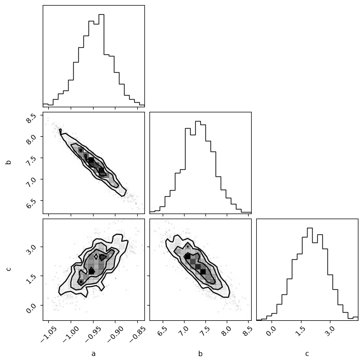
Using this plot, we can visually inspect the marginal posterior distributions for our parameters and get a handle on the parameter uncertainties. Additionally, we can begin to investigate the correlations present between different parameters, e.g., above we can see that a is negatively correlated with b but positively correlated with c.

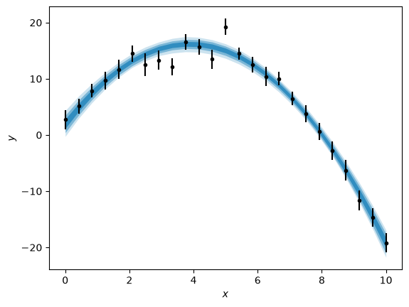
We can also produce a plot showing the posterior distribution of models on the data with a range of credible intervals, shown here with the blue-shaded areas.

credible_intervals = [[16, 84], [2.5, 97.5], [0.15, 99.85]]
alpha = [0.6, 0.4, 0.2]
distribution = flat_samples[:, 0] * x[:, np.newaxis] ** 2 + flat_samples[:, 1] * x[:, np.newaxis] + flat_samples[:, 2]

plt.errorbar(x, y, yerr, marker='.', ls='', color='k')
for i, ci in enumerate(credible_intervals):
    plt.fill_between(x,
                     *np.percentile(distribution, ci, axis=1),
                     alpha=alpha[i],
                     color='#0173B2',
                     lw=0)
plt.xlabel('$x$')
plt.ylabel('$y$')
plt.show()