Thinking about data probabilistically

Thinking about data probabilistically#

Every measurement has some uncertainty associated with it – no measurement is perfect. What causes this uncertainty is not under consideration now, but rather what uncertainty means and how we can think about it in our analysis. Typically, a value with an uncertainty is written as \(\mu \pm \sigma\), where \(\mu\) and \(\sigma\) are the measurement and uncertainty, respectively. While there is (unfortunately) no standard for what this nomenclature means, a common interpretation is that this is describing a normal distribution, which is centred at \(\mu\) with a standard deviation of \(\sigma\) (Fig. 1).

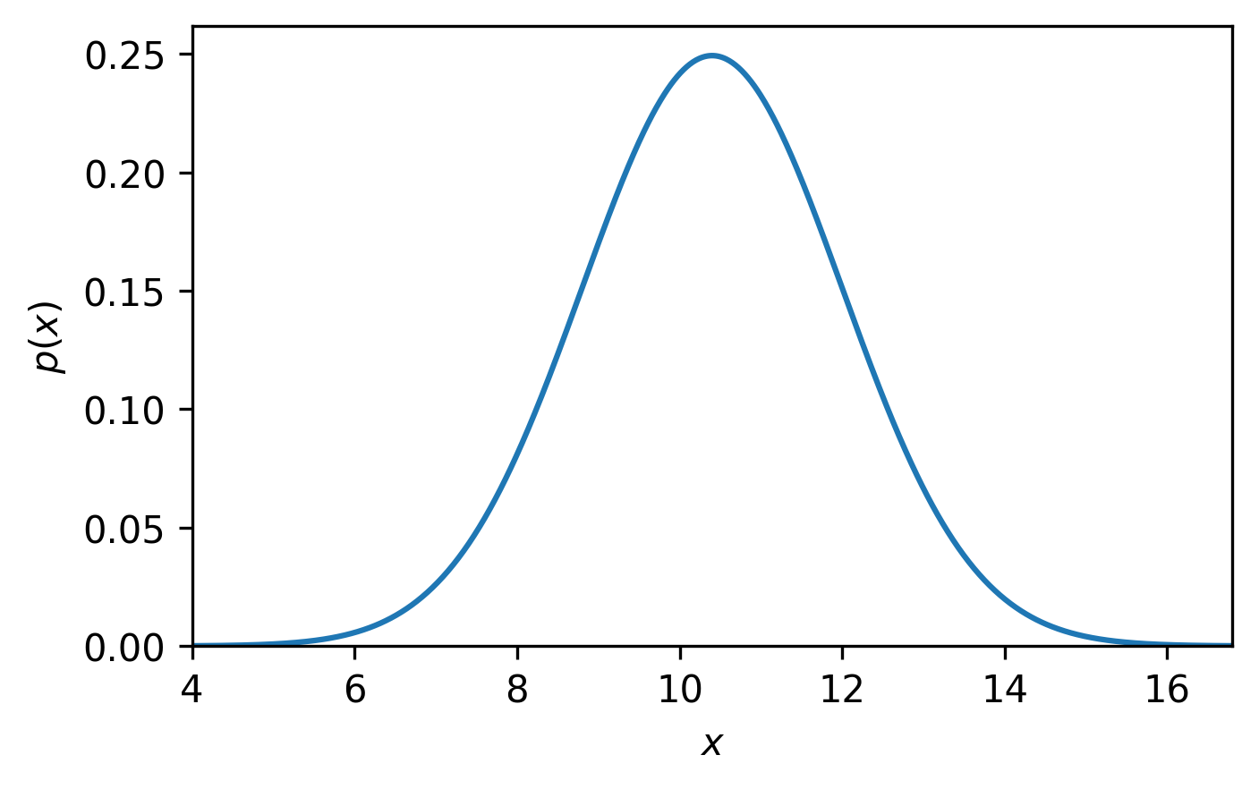
../_images/normal.png — Fig. 1 A normal distribution (blue line), centred on 10.4 with a standard deviation of 1.6.#

Consider the mathematical model \(x=a^2\), that provides a model dataset (of a single data point), where \(a\) is the optimisation parameter[1]. Assume further that we experimentally measured \(x\) to be \(x = \mu \pm \sigma = 10.4 \pm 1.6\) as shown in Fig. 1. The aim of model-dependent analysis is to find the value of \(a\) that leads to the best agreement between our mathematical model and the experimental dataset. Since we assume the measured value to be normally distributed, its probability distribution is

(1)#\[p(x) = \frac{1}{\sigma\sqrt{2\pi}}\exp{\bigg[-\frac{1}{2}\Big(\frac{x-\mu}{\sigma}\Big)^2\bigg]}.\]

\(p\) is called the likelihood of the observation \(\mu \pm \sigma\) given the parameter \(a\). To get the best agreement between the model and the experiment, we need to maximise (or, more commonly, minimise the negative) likelihood. Before passing this task to an optimisation algorithm, we need to have a function that calculates \(-p(x)\) from \(a\), for Eqn. (1).

import numpy as np

mu = 10.4
sigma = 1.6

def nl(a):
    """
    Calculate the negative likelihood for a normal distribution.
    
    Parameters
    ----------
    a: 
        The optimisation parameter, a.
    
    Returns
    -------
    :
        The negative likelihood.
    """
    x = a ** 2
    likelihood = 1 / (sigma * np.sqrt(2 * np.pi)) * np.exp(-0.5 * ((x - mu) / sigma) ** 2)
    return -likelihood

The above function calculates the negative likelihood of a given \(a\) for the data shown in Fig. 1. We can then use the scipy.optimize.minimize optimisation algorithm to minimise this, other minimization libraries are available in Python.

from scipy.optimize import minimize

result = minimize(nl, 2)
print(result)

  message: Optimization terminated successfully.
  success: True
   status: 0
      fun: -0.24933892525083431
        x: [ 3.225e+00]
      nit: 1
      jac: [-6.743e-07]
 hess_inv: [[1]]
     nfev: 24
     njev: 12

The optimisation was successful.

result.success

True

The optimised value of \(a\) was found to be 3.225.

result.x

array([3.22490293])

This result is plotted on top of the data in Fig. 2.

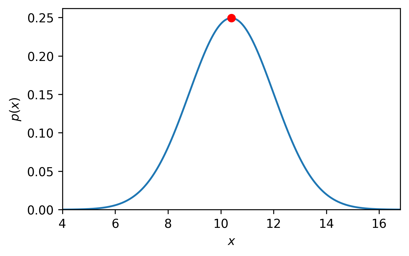
../_images/normal_fit.png — Fig. 2 A normal distribution (blue line), centred on 10.4 with a standard deviation of 1.6 with the maximum likelihood value (red circle).#

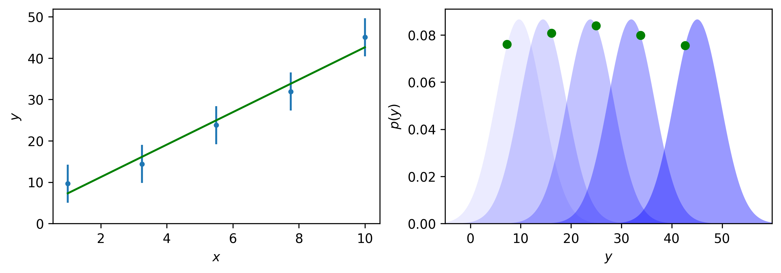
Consider extending this beyond datasets with just a single data point, where each data point is itself a normal distribution. This is visualised in Fig. 3 for five data points; the plot on the left-hand-side presents the data in (hopefully) a familiar way, while the right-hand-side shows the view as though one is sat on the plane of the computer screen, looking along the x-axis.

../_images/multid.png — Fig. 3 Plots with more data points; the standard way to plot data with some uncertainty (e.g., points with error bars) (LHS) and the view of the five likelihood functions for each data point (note that here the uncertainty in each data point is taken to be the same, i.e., it is homoscedastic) (RHS).#

The data in Fig. 3 appears linear, therefore a “straight line fit” can be performed – this is where a gradient and intercept for a straight line (the mathematical model) is found. This results in a model that maximises the product of the likelihoods for each data point, as best as possible given the constraint that the model must hold. It is clear in Fig. 4 that the green model cannot maximise any of the individual distributions, but overall, this is the best possible agreement for the distributions.

../_images/multid_fit.png — Fig. 4 Fig. 3 with a fitted linear model (green).#

This way of thinking about experimental data can be carried through to the use of model-dependent analysis.