Fitting data with easyCore

The easyCore library is designed to enable model-dependent analysis, using a pure Python interface, and give access to a range of optimization algorithms. It is possible to analyse any data for which there is a closed-form mathematical description (i.e., a mathematical model) with parameters to be refined.

This short demonstration will show how easyCore can be used to analyse the toy problem of data following a quadratic relationship. We manufacture some quadratic data to work with below.

Note

easyCore comes packaged with an internal version of numpy that will be used throughout. And we set the random seed to ensure reproducibility in this example.

from easyCore import np

np.random.seed(123)

a_true = -0.9594
b_true = 7.294
c_true = 3.102

N = 25
x = np.linspace(0, 10, N)
yerr = 1 + 1 * np.random.rand(N)
y = a_true * x ** 2 + b_true * x + c_true
y += np.abs(y) * 0.1 * np.random.randn(N)

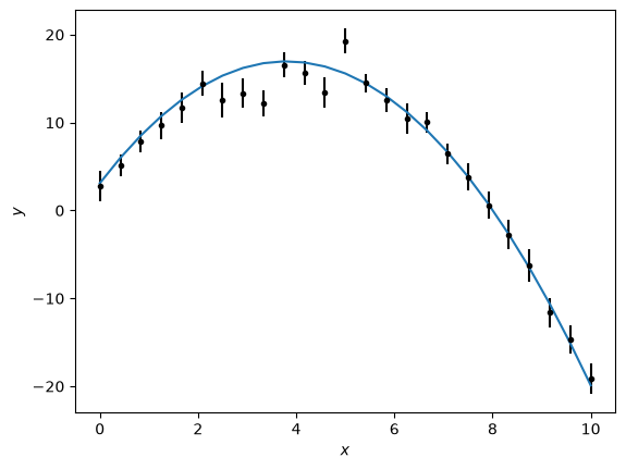
The data created above is shown as a standard error bar plot below.

import matplotlib.pyplot as plt

plt.errorbar(x, y, yerr, marker='.', ls='', color='k')
plt.xlabel('x')
plt.ylabel('y')
plt.show()

The next step is to create an easyCore analysis model. In this example, this consists of three parameters called a, b, and c. These parameters are created and initialised with the true values from above, they are all set with fixed=False as the parameters should be allowed to vary, to find the optimum solution – the only one that maximises the likelihood.

from easyCore.Objects.Variable import Parameter

a = Parameter(name='a', value=a_true, fixed=False)
b = Parameter(name='b', value=b_true, fixed=False)
c = Parameter(name='c', value=c_true, fixed=False)

The mathematical model that is to be optimised is

(2)\[y = a x ^ 2 + b x + c.\]

To use easyCore to optimise this, a Python function that implements this mathematical model is needed.

Note

We use the raw_value property for each parameter in order to get the underlying number and not the parameter object.

We can create a function that implements this mathematical model as shown below.

def math_model(x: np.ndarray) -> np.ndarray:
    """
    Mathematical model for a quadratic. 
    
    :x: values to calculate the model over. 
    
    :return: model values.
    """
    return a.raw_value * x ** 2 + b.raw_value * x + c.raw_value

The initial guess (from the true value) for the mathematical model, along with the experimental data, can then be plotted.

plt.errorbar(x, y, yerr, marker='.', ls='', color='k')
plt.plot(x, math_model(x), '-')
plt.xlabel('$x$')
plt.ylabel('$y$')
plt.show()

To optimise the parameters a, b, and c, a BaseObj must be created. This brings together all parameters to be optimised in a single object, which is then associated with the mathematical model in the Fitter. Note that parameters that are fixed should not be included.

from easyCore.Objects.ObjectClasses import BaseObj
from easyCore.Fitting.Fitting import Fitter

quad = BaseObj(name='quad', a=a, b=b, c=c)
f = Fitter(quad, math_model)

easyCore can then be used to determine the parameters of the quadratic model using maximum likelihood estimation (MLE) . y describes the position of the normal distributions for the data while the weights are the reciprocals of their widths.

res = f.fit(x=x, y=y, weights=1/yerr)

With the MLE found, the parameters can be printed to screen to see the optimized values and estimated statistical uncertainties.

a, b, c

(<Parameter 'a': -0.95+/-0.04, bounds=[-inf:inf]>,
 <Parameter 'b': 7.3+/-0.4, bounds=[-inf:inf]>,
 <Parameter 'c': 2.0+/-0.8, bounds=[-inf:inf]>)

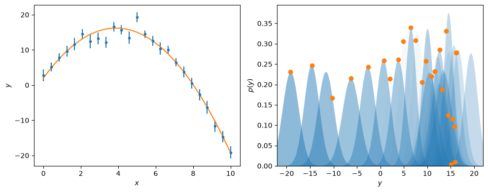
Finally, the optimised model can be plotted with the experimental data, using the same visualisation as previously.

from scipy.stats import norm

fig, ax = plt.subplots(1, 2, figsize=(10, 4))

ax[0].errorbar(x, y, yerr, marker='.', ls='', color='C0')
ax[0].plot(x, math_model(x), '-', color='C1')
ax[0].set_xlabel('$x$')
ax[0].set_ylabel('$y$')

y_range = np.arange(-22, 22, 0.1)
for i, yy in enumerate(y):
    ax[1].fill_between(y_range, norm(yy, yerr[i]).pdf(y_range), color='C0', alpha=0.02 * (i + 1), lw=0)
    ax[1].plot(math_model(x[i]), norm(yy, yerr[i]).pdf(math_model(x[i])), 'C1o')
ax[1].set_xlim(y_range.min(), y_range.max())
ax[1].set_ylim(0, None)
ax[1].set_xlabel('$y$')
ax[1].set_ylabel('$p(y)$')
plt.tight_layout()
plt.show()

This approach to use easyCore for the optimization of mathematical models can be applied to many different use cases, including in neutron scattering.