Introduction to Sciline#
Data processing workflow management tool.
scipp.github.io/sciline/
It is worth taking your time going through this notebook, do not try to rush it.
Sciline is an open-source library developed by ESS for managing and visualizing data processing workflows (sometimes called “pipelines”).
It defines workflows as directed acyclic graphs (DAGs) where the nodes are inputs, intermediate results, or final results, and edges are dependencies between the nodes.
This has some benefits:
Any (named) intermediate result in the pipeline can be computed.
The dependencies between intermediate results can be visualized.
Implementations of intermediate result can be replaced.
Results that are expensive to compute can be cached.
Certainty that the computed result has not been corrupted by running jupyter cells out of order.
Terminology#
A Sciline workflow (or “pipeline”) is defined by a set of transformations or providers that specify what inputs are needed to compute one specific output quantity.
The input and output quantities of the providers are called domain types.
A provider is a python function with type annotations:
# Example provider
def load_run(
    run_number: RunNumber,
    proposal_number: ProposalNumber,
    data_dir_path: DataPath,
) -> LoadedNexusData:

    filename = f'{proposal_number}_{run_number:06d}.hdf'
    path = os.path.join(data_dir_path, filename)

    data = scippnexus.load(path)

    return data
In the above example, to compute the LoadedNexusData quantity the RunNumber, ProposalNumber and the DataPath quantities are needed.
LoadedNexusData, RunNumber, ProposalNumber and DataPath are “domain types”.
The domain types are the nodes in the workflow graph, and they represent the inputs, intermediate results, or final results of the workflow.
Inputs, intermediate results, and final results#
A typical data reduction workflow has some “Inputs”, some “Intermediate results” and some “Final results”.
Sciline does not distinguish between those, but it is useful to make a loose distinction:
Inputs are typically:
The name of one or more NeXus files.
Parameters defining a region of interest (ROI),
for example the wavelength range.
The number of histogram bins.
Intermediate results are typically:
List of events with associated coordinates, masks, and weights.
“Coordinates” such as wavelength, scattering angle, etc.
Monitor wavelength histogram.
Various calibration factors that are computed or loaded from file.
Final results are typically:
Curve describing the scattering cross section \(S(Q)\) as a function of momentum transfer (SANS).
List of peaks and associated intensities (diffraction).
Etc.

How does Sciline know how to build the graph?#
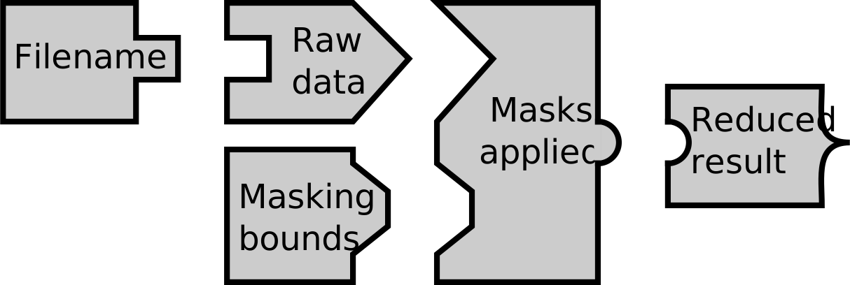
Each domain type is unique, and given a list of all functions to be used in the workflow, Sciline can figure out how to connect the nodes in the graph.
Think of it like puzzle pieces that fit into each other:

Example#
import os
from typing import NewType

import sciline as sl
import scipp as sc

from scippneutron.conversion.graph.beamline import beamline
from scippneutron.conversion.graph.tof import elastic

import sans_utils as utils

graph = {**beamline(scatter=True), **elastic("tof")}
Creating a pipeline#
We start by by defining the domain types: the quantities representing input parameters, intermediate results and the final results of the pipeline.
Foldername = NewType("Foldername", str)
"""Folder name for measurements."""

RawData = NewType("RawData", sc.DataArray)
"""Raw loaded data."""

CoordTransformGraph = NewType("CoordTransformGraph", dict)
"""Graph describing coordinate transformations."""

WavelengthData = NewType("WavelengthData", sc.DataArray)
"""Data with wavelength coordinate."""

QData = NewType("Qdata", sc.DataArray)
"""Data with Q coordinate."""

QBins = NewType("QBins", sc.Variable)
"""Bin edges in the Q dimension."""

QHistogram = NewType("QHistogram", sc.DataArray)
"""Data histogrammed in Q bins."""
Next, we create the ‘provider’ functions: the operations that determine how do we get from one domain type to the next.
def load(folder: Foldername) -> RawData:
    """Load raw data from file"""
    return utils.load_sans(folder)


def to_wavelength(data: RawData, graph: CoordTransformGraph) -> WavelengthData:
    """Compute wavelength for events"""
    return data.transform_coords("wavelength", graph=graph)


def to_Q(data: WavelengthData, graph: CoordTransformGraph) -> QData:
    """Compute Q for events"""
    return data.transform_coords("Q", graph=graph)


def to_histogram(events: QData, qbins: QBins) -> QHistogram:
    """Histogram data in Q bins"""
    return events.hist(Q=qbins)
Finally, we build the workflow (also known as a ‘pipeline’) by supplying the list of our functions defined above:
workflow = sl.Pipeline(
    # List the providers that make up the workflow.
    (load, to_wavelength, to_Q, to_histogram),
)

workflow.visualize(graph_attr={"rankdir": "LR"})

Some domain types are visualized in red color and with dashed border, those are the domain types that lack a definition.
Setting parameters#
To set a parameter on the workflow, we use the setitem operator [] (as one would do with a python dict):
workflow[QBins] = sc.linspace("Q", 5.0e-3, 0.19, 201, unit="1/angstrom")
workflow[Foldername] = utils.fetch_data("3-mcstas/SANS_with_sample")
workflow[CoordTransformGraph] = graph
We can now visualize the workflow again and see that the red boxes have now turned black;
all parameters required to compute the QHistogram have been set.
workflow.visualize(graph_attr={"rankdir": "LR"})

Computing quantities#
Until now, not computations have taken place. We have simply set-up the framework for the reduction in the shape of a task-graph, but nothing has been computed yet.
Building and manipulating the graph is very cheap, and only once we are satisfied with it should we then proceed with computing the final result.
This is done by calling the compute method:
q_hist = workflow.compute(QHistogram)
q_hist
- Q: 200
- L1()float64m150.0
Values:
array(150.) - Q(Q [bin-edge])float641/Å0.005, 0.006, ..., 0.189, 0.19
Values:
array([0.005 , 0.005925, 0.00685 , 0.007775, 0.0087 , 0.009625, 0.01055 , 0.011475, 0.0124 , 0.013325, 0.01425 , 0.015175, 0.0161 , 0.017025, 0.01795 , 0.018875, 0.0198 , 0.020725, 0.02165 , 0.022575, 0.0235 , 0.024425, 0.02535 , 0.026275, 0.0272 , 0.028125, 0.02905 , 0.029975, 0.0309 , 0.031825, 0.03275 , 0.033675, 0.0346 , 0.035525, 0.03645 , 0.037375, 0.0383 , 0.039225, 0.04015 , 0.041075, 0.042 , 0.042925, 0.04385 , 0.044775, 0.0457 , 0.046625, 0.04755 , 0.048475, 0.0494 , 0.050325, 0.05125 , 0.052175, 0.0531 , 0.054025, 0.05495 , 0.055875, 0.0568 , 0.057725, 0.05865 , 0.059575, 0.0605 , 0.061425, 0.06235 , 0.063275, 0.0642 , 0.065125, 0.06605 , 0.066975, 0.0679 , 0.068825, 0.06975 , 0.070675, 0.0716 , 0.072525, 0.07345 , 0.074375, 0.0753 , 0.076225, 0.07715 , 0.078075, 0.079 , 0.079925, 0.08085 , 0.081775, 0.0827 , 0.083625, 0.08455 , 0.085475, 0.0864 , 0.087325, 0.08825 , 0.089175, 0.0901 , 0.091025, 0.09195 , 0.092875, 0.0938 , 0.094725, 0.09565 , 0.096575, 0.0975 , 0.098425, 0.09935 , 0.100275, 0.1012 , 0.102125, 0.10305 , 0.103975, 0.1049 , 0.105825, 0.10675 , 0.107675, 0.1086 , 0.109525, 0.11045 , 0.111375, 0.1123 , 0.113225, 0.11415 , 0.115075, 0.116 , 0.116925, 0.11785 , 0.118775, 0.1197 , 0.120625, 0.12155 , 0.122475, 0.1234 , 0.124325, 0.12525 , 0.126175, 0.1271 , 0.128025, 0.12895 , 0.129875, 0.1308 , 0.131725, 0.13265 , 0.133575, 0.1345 , 0.135425, 0.13635 , 0.137275, 0.1382 , 0.139125, 0.14005 , 0.140975, 0.1419 , 0.142825, 0.14375 , 0.144675, 0.1456 , 0.146525, 0.14745 , 0.148375, 0.1493 , 0.150225, 0.15115 , 0.152075, 0.153 , 0.153925, 0.15485 , 0.155775, 0.1567 , 0.157625, 0.15855 , 0.159475, 0.1604 , 0.161325, 0.16225 , 0.163175, 0.1641 , 0.165025, 0.16595 , 0.166875, 0.1678 , 0.168725, 0.16965 , 0.170575, 0.1715 , 0.172425, 0.17335 , 0.174275, 0.1752 , 0.176125, 0.17705 , 0.177975, 0.1789 , 0.179825, 0.18075 , 0.181675, 0.1826 , 0.183525, 0.18445 , 0.185375, 0.1863 , 0.187225, 0.18815 , 0.189075, 0.19 ]) - incident_beam()vector3m[ 0. 0. 150.]
Values:
array([ 0., 0., 150.]) - sample_position()vector3m[0. 0. 0.]
Values:
array([0., 0., 0.]) - source_position()vector3m[ 0. 0. -150.]
Values:
array([   0.,    0., -150.])
- (Q)float64counts2651.198, 4083.465, ..., 0.285, 0.058σ = 58.679, 82.257, ..., 0.107, 0.017
Values:
array([2.65119769e+03, 4.08346496e+03, 4.04656525e+03, 3.76836977e+03,
       3.78803031e+03, 3.55300298e+03, 3.55454343e+03, 3.36962136e+03,
       3.30428426e+03, 3.03903095e+03, 2.85846287e+03, 2.95314414e+03,
       2.76133429e+03, 2.55496452e+03, 2.23378971e+03, 2.14013675e+03,
       1.81911835e+03, 1.72271870e+03, 1.45409208e+03, 1.31687287e+03,
       9.86107823e+02, 8.08752540e+02, 8.15756917e+02, 7.91374374e+02,
       5.65775045e+02, 5.72131167e+02, 5.50137127e+02, 4.36450418e+02,
       4.41282615e+02, 3.91479858e+02, 2.76073319e+02, 2.46873547e+02,
       2.30193487e+02, 2.34714835e+02, 1.60073544e+02, 1.20309146e+02,
       1.20438966e+02, 7.82021509e+01, 6.90773315e+01, 5.99165814e+01,
       5.24179420e+01, 4.81731116e+01, 2.89452212e+01, 2.80461625e+01,
       2.79078145e+01, 2.13982527e+01, 2.02352269e+01, 1.77034814e+01,
       1.54255362e+01, 2.13855704e+01, 1.88464775e+01, 2.53235388e+01,
       2.82173046e+01, 2.85258966e+01, 3.29145914e+01, 2.52613854e+01,
       4.15131086e+01, 2.94660375e+01, 4.76172615e+01, 3.57778718e+01,
       4.69193593e+01, 3.41692979e+01, 4.29265616e+01, 4.54020919e+01,
       4.29084156e+01, 4.33820462e+01, 4.78897422e+01, 3.95390928e+01,
       3.75110151e+01, 3.67323272e+01, 4.44719361e+01, 4.12794851e+01,
       3.68472257e+01, 3.05493263e+01, 2.95380881e+01, 2.41500777e+01,
       3.05556449e+01, 2.25663693e+01, 1.87464908e+01, 1.76881667e+01,
       2.03162662e+01, 1.84117878e+01, 1.32340948e+01, 1.57129644e+01,
       1.80801172e+01, 1.64953047e+01, 1.58660859e+01, 1.53366396e+01,
       1.91896327e+01, 1.87668355e+01, 1.65085122e+01, 1.51991354e+01,
       2.01371082e+01, 2.04383997e+01, 1.45280133e+01, 1.94384106e+01,
       2.30164734e+01, 1.64857239e+01, 1.56442119e+01, 2.01837331e+01,
       2.39511850e+01, 1.63154185e+01, 1.96870027e+01, 2.24737182e+01,
       2.23868140e+01, 1.81285375e+01, 2.23357293e+01, 2.13357717e+01,
       1.90930230e+01, 2.03574012e+01, 1.48672001e+01, 2.06191466e+01,
       1.48149382e+01, 1.46696980e+01, 1.69822433e+01, 1.92685251e+01,
       1.59816537e+01, 1.60240048e+01, 1.61214459e+01, 1.71844158e+01,
       1.35419967e+01, 1.21652682e+01, 1.61160226e+01, 1.33476057e+01,
       1.82490925e+01, 1.52357099e+01, 1.71350700e+01, 1.29610232e+01,
       1.36145515e+01, 1.27754972e+01, 1.70184243e+01, 1.71933264e+01,
       1.09889571e+01, 2.06088233e+01, 1.41275969e+01, 1.50999561e+01,
       1.40828223e+01, 1.10066356e+01, 2.56253080e+01, 1.29470789e+01,
       1.75901912e+01, 1.67824633e+01, 1.34531005e+01, 1.68673359e+01,
       1.86151535e+01, 1.84008493e+01, 1.50575232e+01, 1.60010708e+01,
       1.68956606e+01, 1.59628359e+01, 2.09781944e+01, 1.71699325e+01,
       1.27948650e+01, 1.55163191e+01, 1.08730150e+01, 1.06797968e+01,
       1.12020380e+01, 1.03572306e+01, 9.16162899e+00, 1.38442839e+01,
       1.36081269e+01, 1.06322920e+01, 1.06591682e+01, 2.33180798e+01,
       8.54705642e+00, 1.01454104e+01, 1.08536824e+01, 1.00587952e+01,
       1.29653450e+01, 1.15495310e+01, 1.10632017e+01, 1.06491463e+01,
       1.05646625e+01, 1.16623350e+01, 5.67695377e+00, 1.11328288e+01,
       9.87699426e+00, 5.78032493e+00, 4.31319524e+00, 4.46777002e+00,
       7.77070601e+00, 7.38907133e+00, 6.69735623e+00, 4.43288956e+00,
       6.30950161e+00, 6.85855864e+00, 4.99187265e+00, 3.69753928e+00,
       7.69471655e+00, 2.07439494e+00, 3.97213700e+00, 3.40678827e+00,
       1.21622902e+00, 1.34470708e+00, 8.03492359e-01, 2.34978789e+00,
       2.35761800e+00, 2.61321639e-01, 2.84620549e-01, 5.77960665e-02])

Variances (σ²):
array([3.44318428e+03, 6.76614232e+03, 7.57401233e+03, 7.95824880e+03,
       9.18995394e+03, 9.57373825e+03, 1.06207859e+04, 1.07856850e+04,
       1.19534993e+04, 1.16201321e+04, 1.17709297e+04, 1.29856678e+04,
       1.28617142e+04, 1.20372733e+04, 1.08421687e+04, 1.11272160e+04,
       9.46586345e+03, 9.36149369e+03, 8.01182169e+03, 7.17230861e+03,
       5.33496358e+03, 4.03947409e+03, 4.19579357e+03, 4.00328876e+03,
       2.64009542e+03, 2.53333030e+03, 2.51767095e+03, 1.82043323e+03,
       1.73441815e+03, 1.45585612e+03, 8.88946762e+02, 7.71768252e+02,
       6.36919759e+02, 6.51105889e+02, 3.50543479e+02, 2.46709601e+02,
       2.09339687e+02, 1.07244231e+02, 7.65068283e+01, 5.46381519e+01,
       4.11343749e+01, 3.53414746e+01, 1.34336181e+01, 1.15037434e+01,
       8.20598676e+00, 4.25039054e+00, 3.01124336e+00, 2.46798995e+00,
       2.01159229e+00, 3.71923251e+00, 3.39813450e+00, 7.04173369e+00,
       9.21325375e+00, 1.06655865e+01, 1.30446401e+01, 9.05497428e+00,
       2.33478515e+01, 1.65388230e+01, 3.29726758e+01, 2.19573147e+01,
       3.78132540e+01, 2.44362133e+01, 3.43053854e+01, 3.65895300e+01,
       3.62331273e+01, 3.66718310e+01, 3.81700885e+01, 3.12644239e+01,
       2.80907050e+01, 2.67870999e+01, 3.33219593e+01, 3.29296240e+01,
       2.43768982e+01, 1.78451130e+01, 1.60312652e+01, 1.05488288e+01,
       1.67323543e+01, 8.67295661e+00, 6.21470312e+00, 5.09204193e+00,
       6.09906864e+00, 5.75444682e+00, 2.08661595e+00, 3.16321417e+00,
       4.32130874e+00, 3.79564137e+00, 3.34115074e+00, 3.97181410e+00,
       4.88196914e+00, 4.96265132e+00, 4.55681470e+00, 3.86712090e+00,
       6.94756104e+00, 7.85574070e+00, 4.74011774e+00, 8.74198896e+00,
       1.05707711e+01, 6.81388339e+00, 6.95511118e+00, 9.49984032e+00,
       1.43769608e+01, 6.54791387e+00, 1.06403477e+01, 1.21901993e+01,
       1.37120708e+01, 8.51742879e+00, 1.39973536e+01, 1.33538325e+01,
       9.50335662e+00, 1.03030521e+01, 5.41231791e+00, 1.03580736e+01,
       5.03099652e+00, 4.83712164e+00, 7.48411157e+00, 8.47968446e+00,
       6.73434966e+00, 5.79650910e+00, 6.46251438e+00, 6.57683203e+00,
       5.47663233e+00, 3.87571428e+00, 6.95513166e+00, 4.21646716e+00,
       9.30980772e+00, 6.68686531e+00, 8.23806748e+00, 5.41265859e+00,
       5.19673675e+00, 5.72729329e+00, 1.03744585e+01, 9.44153823e+00,
       3.91976324e+00, 1.32199293e+01, 6.19020312e+00, 9.48319189e+00,
       6.35687894e+00, 4.05867131e+00, 2.02379236e+01, 7.13018558e+00,
       1.13072834e+01, 1.18468588e+01, 8.48998000e+00, 1.25570228e+01,
       1.33723677e+01, 1.35024445e+01, 7.94978063e+00, 1.11747226e+01,
       9.78271925e+00, 1.18082338e+01, 1.66867589e+01, 1.02908398e+01,
       7.17454790e+00, 1.07847468e+01, 3.22217046e+00, 3.69509977e+00,
       4.83713434e+00, 4.69206863e+00, 1.78514854e+00, 5.73411767e+00,
       1.03845205e+01, 5.81308022e+00, 4.79541510e+00, 2.39950198e+01,
       3.20333923e+00, 6.56482395e+00, 7.53416699e+00, 7.37680422e+00,
       1.10252136e+01, 9.46078465e+00, 1.04917959e+01, 8.39225133e+00,
       8.23748654e+00, 1.01111658e+01, 3.18475693e+00, 1.21967818e+01,
       8.77616229e+00, 2.53928688e+00, 1.05634761e+00, 1.69813640e+00,
       9.11773445e+00, 8.32106832e+00, 4.09806132e+00, 4.53704010e+00,
       9.15017317e+00, 9.32920970e+00, 3.25571913e+00, 1.33831391e+00,
       9.96604380e+00, 1.30829447e-01, 4.90941107e+00, 3.52723959e+00,
       6.13495275e-02, 8.11932922e-02, 3.59332436e-02, 3.41202988e+00,
       3.36091085e+00, 3.34791666e-03, 1.13889333e-02, 2.75568783e-04])
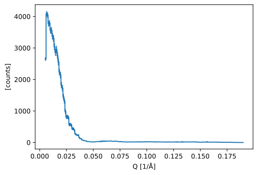
q_hist.plot()
Intermediate results#
One of the most powerful features about sciline is that once we have built a graph,
any step (node) in the graph can be inspected.
This is extremely useful for looking at intermediate results, while debugging a workflow for instance.
Computing intermediate results is also done with the compute method, but we simply pass as the argument the type that corresponds to the quantity we wish to compute.
wavelength_data = workflow.compute(WavelengthData)
wavelength_data
- event: 6797906
- L1()float64m150.0
Values:
array(150.) - L2(event)float64m3.011, 3.011, ..., 3.013, 3.013
Values:
array([3.01096078, 3.01088826, 3.01079939, ..., 3.01318204, 3.01319606, 3.01308443], shape=(6797906,)) - Ltotal(event)float64m153.011, 153.011, ..., 153.013, 153.013
Values:
array([153.01096078, 153.01088826, 153.01079939, ..., 153.01318204, 153.01319606, 153.01308443], shape=(6797906,)) - incident_beam()vector3m[ 0. 0. 150.]
Values:
array([ 0., 0., 150.]) - position(event)vector3m[0. 0.25668036 3. ], [0. 0.25582825 3. ], ..., [0. 0.28169222 3. ], [0. 0.2804956 3. ]
Values:
array([[0. , 0.25668036, 3. ], [0. , 0.25582825, 3. ], [0. , 0.25478019, 3. ], ..., [0. , 0.2815422 , 3. ], [0. , 0.28169222, 3. ], [0. , 0.2804956 , 3. ]], shape=(6797906, 3)) - sample_position()vector3m[0. 0. 0.]
Values:
array([0., 0., 0.]) - scattered_beam(event)vector3m[0. 0.25668036 3. ], [0. 0.25582825 3. ], ..., [0. 0.28169222 3. ], [0. 0.2804956 3. ]
Values:
array([[0. , 0.25668036, 3. ], [0. , 0.25582825, 3. ], [0. , 0.25478019, 3. ], ..., [0. , 0.2815422 , 3. ], [0. , 0.28169222, 3. ], [0. , 0.2804956 , 3. ]], shape=(6797906, 3)) - source_position()vector3m[ 0. 0. -150.]
Values:
array([ 0., 0., -150.]) - tof(event)float64ms257.339, 257.341, ..., 241.356, 241.364
Values:
array([257.33946994, 257.34093926, 257.34306265, ..., 241.35329852, 241.35588096, 241.36409091], shape=(6797906,)) - wavelength(event)float64Å6.653, 6.653, ..., 6.240, 6.240
Values:
array([6.65340371, 6.65344485, 6.65350362, ..., 6.23999739, 6.24006358, 6.2402804 ], shape=(6797906,)) - x(event)float64m0.0, 0.0, ..., 0.0, 0.0
Values:
array([0., 0., 0., ..., 0., 0., 0.], shape=(6797906,)) - y(event)float64m0.257, 0.256, ..., 0.282, 0.280
Values:
array([0.25668036, 0.25582825, 0.25478019, ..., 0.2815422 , 0.28169222,
       0.2804956 ], shape=(6797906,))
- (event)float64counts1.488e-17, 1.244e-21, ..., 1.385e-59, 1.210e-63σ = 1.488e-17, 1.244e-21, ..., 1.385e-59, 1.210e-63
Values:
array([1.48840676e-17, 1.24410115e-21, 1.03989562e-25, ...,
       1.58397338e-55, 1.38453144e-59, 1.21020172e-63], shape=(6797906,))

Variances (σ²):
array([2.21535468e-034, 1.54778768e-042, 1.08138291e-050, ...,
       2.50897168e-110, 1.91692732e-118, 1.46458821e-126],
      shape=(6797906,))
Computing multiple results#
It is also possible to request more than one result in one go.
This is useful because whenever we compute a quantity, sciline walks the entire graph all over again; nothing is cached.
This default behaviour ensures the correctness and reproducibility of results.
So when we first computed the QHistogram and then the WavelengthData above in 2 separate compute calls,
we actually loaded the file twice.
To avoid this, we can request both targets inside the call to compute, and the file will only be loaded once (the scheduler will identify which parts of the graph are needed for which result and will not repeat branches used by both).
two_results = workflow.compute((WavelengthData, QHistogram))
two_results
{__main__.WavelengthData: <scipp.DataArray>
 Dimensions: Sizes[event:6797906, ]
 Coordinates:
   L1                        float64              [m]  ()  150
   L2                        float64              [m]  (event)  [3.01096, 3.01089, ..., 3.0132, 3.01308]
   Ltotal                    float64              [m]  (event)  [153.011, 153.011, ..., 153.013, 153.013]
   incident_beam             vector3              [m]  ()  (0, 0, 150)
   position                  vector3              [m]  (event)  [(0, 0.25668, 3), (0, 0.255828, 3), ..., (0, 0.281692, 3), (0, 0.280496, 3)]
   sample_position           vector3              [m]  ()  (0, 0, 0)
   scattered_beam            vector3              [m]  (event)  [(0, 0.25668, 3), (0, 0.255828, 3), ..., (0, 0.281692, 3), (0, 0.280496, 3)]
   source_position           vector3              [m]  ()  (0, 0, -150)
   tof                       float64             [ms]  (event)  [257.339, 257.341, ..., 241.356, 241.364]
 * wavelength                float64             [Å]  (event)  [6.6534, 6.65344, ..., 6.24006, 6.24028]
 * x                         float64              [m]  (event)  [0, 0, ..., 0, 0]
 * y                         float64              [m]  (event)  [0.25668, 0.255828, ..., 0.281692, 0.280496]
 Data:
                             float64         [counts]  (event)  [1.48841e-17, 1.2441e-21, ..., 1.38453e-59, 1.2102e-63]  [2.21535e-34, 1.54779e-42, ..., 1.91693e-118, 1.46459e-126]
 ,
 __main__.QHistogram: <scipp.DataArray>
 Dimensions: Sizes[Q:200, ]
 Coordinates:
   L1                        float64              [m]  ()  150
 * Q                         float64           [1/Å]  (Q [bin-edge])  [0.005, 0.005925, ..., 0.189075, 0.19]
   incident_beam             vector3              [m]  ()  (0, 0, 150)
   sample_position           vector3              [m]  ()  (0, 0, 0)
   source_position           vector3              [m]  ()  (0, 0, -150)
 Data:
                             float64         [counts]  (Q)  [2651.2, 4083.46, ..., 0.284621, 0.0577961]  [3443.18, 6766.14, ..., 0.0113889, 0.000275569]
 }
The results are stored in a dictionary where the keys are just the requested types:
two_results[QHistogram]
- Q: 200
- L1()float64m150.0
Values:
array(150.) - Q(Q [bin-edge])float641/Å0.005, 0.006, ..., 0.189, 0.19
Values:
array([0.005 , 0.005925, 0.00685 , 0.007775, 0.0087 , 0.009625, 0.01055 , 0.011475, 0.0124 , 0.013325, 0.01425 , 0.015175, 0.0161 , 0.017025, 0.01795 , 0.018875, 0.0198 , 0.020725, 0.02165 , 0.022575, 0.0235 , 0.024425, 0.02535 , 0.026275, 0.0272 , 0.028125, 0.02905 , 0.029975, 0.0309 , 0.031825, 0.03275 , 0.033675, 0.0346 , 0.035525, 0.03645 , 0.037375, 0.0383 , 0.039225, 0.04015 , 0.041075, 0.042 , 0.042925, 0.04385 , 0.044775, 0.0457 , 0.046625, 0.04755 , 0.048475, 0.0494 , 0.050325, 0.05125 , 0.052175, 0.0531 , 0.054025, 0.05495 , 0.055875, 0.0568 , 0.057725, 0.05865 , 0.059575, 0.0605 , 0.061425, 0.06235 , 0.063275, 0.0642 , 0.065125, 0.06605 , 0.066975, 0.0679 , 0.068825, 0.06975 , 0.070675, 0.0716 , 0.072525, 0.07345 , 0.074375, 0.0753 , 0.076225, 0.07715 , 0.078075, 0.079 , 0.079925, 0.08085 , 0.081775, 0.0827 , 0.083625, 0.08455 , 0.085475, 0.0864 , 0.087325, 0.08825 , 0.089175, 0.0901 , 0.091025, 0.09195 , 0.092875, 0.0938 , 0.094725, 0.09565 , 0.096575, 0.0975 , 0.098425, 0.09935 , 0.100275, 0.1012 , 0.102125, 0.10305 , 0.103975, 0.1049 , 0.105825, 0.10675 , 0.107675, 0.1086 , 0.109525, 0.11045 , 0.111375, 0.1123 , 0.113225, 0.11415 , 0.115075, 0.116 , 0.116925, 0.11785 , 0.118775, 0.1197 , 0.120625, 0.12155 , 0.122475, 0.1234 , 0.124325, 0.12525 , 0.126175, 0.1271 , 0.128025, 0.12895 , 0.129875, 0.1308 , 0.131725, 0.13265 , 0.133575, 0.1345 , 0.135425, 0.13635 , 0.137275, 0.1382 , 0.139125, 0.14005 , 0.140975, 0.1419 , 0.142825, 0.14375 , 0.144675, 0.1456 , 0.146525, 0.14745 , 0.148375, 0.1493 , 0.150225, 0.15115 , 0.152075, 0.153 , 0.153925, 0.15485 , 0.155775, 0.1567 , 0.157625, 0.15855 , 0.159475, 0.1604 , 0.161325, 0.16225 , 0.163175, 0.1641 , 0.165025, 0.16595 , 0.166875, 0.1678 , 0.168725, 0.16965 , 0.170575, 0.1715 , 0.172425, 0.17335 , 0.174275, 0.1752 , 0.176125, 0.17705 , 0.177975, 0.1789 , 0.179825, 0.18075 , 0.181675, 0.1826 , 0.183525, 0.18445 , 0.185375, 0.1863 , 0.187225, 0.18815 , 0.189075, 0.19 ]) - incident_beam()vector3m[ 0. 0. 150.]
Values:
array([ 0., 0., 150.]) - sample_position()vector3m[0. 0. 0.]
Values:
array([0., 0., 0.]) - source_position()vector3m[ 0. 0. -150.]
Values:
array([   0.,    0., -150.])
- (Q)float64counts2651.198, 4083.465, ..., 0.285, 0.058σ = 58.679, 82.257, ..., 0.107, 0.017
Values:
array([2.65119769e+03, 4.08346496e+03, 4.04656525e+03, 3.76836977e+03,
       3.78803031e+03, 3.55300298e+03, 3.55454343e+03, 3.36962136e+03,
       3.30428426e+03, 3.03903095e+03, 2.85846287e+03, 2.95314414e+03,
       2.76133429e+03, 2.55496452e+03, 2.23378971e+03, 2.14013675e+03,
       1.81911835e+03, 1.72271870e+03, 1.45409208e+03, 1.31687287e+03,
       9.86107823e+02, 8.08752540e+02, 8.15756917e+02, 7.91374374e+02,
       5.65775045e+02, 5.72131167e+02, 5.50137127e+02, 4.36450418e+02,
       4.41282615e+02, 3.91479858e+02, 2.76073319e+02, 2.46873547e+02,
       2.30193487e+02, 2.34714835e+02, 1.60073544e+02, 1.20309146e+02,
       1.20438966e+02, 7.82021509e+01, 6.90773315e+01, 5.99165814e+01,
       5.24179420e+01, 4.81731116e+01, 2.89452212e+01, 2.80461625e+01,
       2.79078145e+01, 2.13982527e+01, 2.02352269e+01, 1.77034814e+01,
       1.54255362e+01, 2.13855704e+01, 1.88464775e+01, 2.53235388e+01,
       2.82173046e+01, 2.85258966e+01, 3.29145914e+01, 2.52613854e+01,
       4.15131086e+01, 2.94660375e+01, 4.76172615e+01, 3.57778718e+01,
       4.69193593e+01, 3.41692979e+01, 4.29265616e+01, 4.54020919e+01,
       4.29084156e+01, 4.33820462e+01, 4.78897422e+01, 3.95390928e+01,
       3.75110151e+01, 3.67323272e+01, 4.44719361e+01, 4.12794851e+01,
       3.68472257e+01, 3.05493263e+01, 2.95380881e+01, 2.41500777e+01,
       3.05556449e+01, 2.25663693e+01, 1.87464908e+01, 1.76881667e+01,
       2.03162662e+01, 1.84117878e+01, 1.32340948e+01, 1.57129644e+01,
       1.80801172e+01, 1.64953047e+01, 1.58660859e+01, 1.53366396e+01,
       1.91896327e+01, 1.87668355e+01, 1.65085122e+01, 1.51991354e+01,
       2.01371082e+01, 2.04383997e+01, 1.45280133e+01, 1.94384106e+01,
       2.30164734e+01, 1.64857239e+01, 1.56442119e+01, 2.01837331e+01,
       2.39511850e+01, 1.63154185e+01, 1.96870027e+01, 2.24737182e+01,
       2.23868140e+01, 1.81285375e+01, 2.23357293e+01, 2.13357717e+01,
       1.90930230e+01, 2.03574012e+01, 1.48672001e+01, 2.06191466e+01,
       1.48149382e+01, 1.46696980e+01, 1.69822433e+01, 1.92685251e+01,
       1.59816537e+01, 1.60240048e+01, 1.61214459e+01, 1.71844158e+01,
       1.35419967e+01, 1.21652682e+01, 1.61160226e+01, 1.33476057e+01,
       1.82490925e+01, 1.52357099e+01, 1.71350700e+01, 1.29610232e+01,
       1.36145515e+01, 1.27754972e+01, 1.70184243e+01, 1.71933264e+01,
       1.09889571e+01, 2.06088233e+01, 1.41275969e+01, 1.50999561e+01,
       1.40828223e+01, 1.10066356e+01, 2.56253080e+01, 1.29470789e+01,
       1.75901912e+01, 1.67824633e+01, 1.34531005e+01, 1.68673359e+01,
       1.86151535e+01, 1.84008493e+01, 1.50575232e+01, 1.60010708e+01,
       1.68956606e+01, 1.59628359e+01, 2.09781944e+01, 1.71699325e+01,
       1.27948650e+01, 1.55163191e+01, 1.08730150e+01, 1.06797968e+01,
       1.12020380e+01, 1.03572306e+01, 9.16162899e+00, 1.38442839e+01,
       1.36081269e+01, 1.06322920e+01, 1.06591682e+01, 2.33180798e+01,
       8.54705642e+00, 1.01454104e+01, 1.08536824e+01, 1.00587952e+01,
       1.29653450e+01, 1.15495310e+01, 1.10632017e+01, 1.06491463e+01,
       1.05646625e+01, 1.16623350e+01, 5.67695377e+00, 1.11328288e+01,
       9.87699426e+00, 5.78032493e+00, 4.31319524e+00, 4.46777002e+00,
       7.77070601e+00, 7.38907133e+00, 6.69735623e+00, 4.43288956e+00,
       6.30950161e+00, 6.85855864e+00, 4.99187265e+00, 3.69753928e+00,
       7.69471655e+00, 2.07439494e+00, 3.97213700e+00, 3.40678827e+00,
       1.21622902e+00, 1.34470708e+00, 8.03492359e-01, 2.34978789e+00,
       2.35761800e+00, 2.61321639e-01, 2.84620549e-01, 5.77960665e-02])

Variances (σ²):
array([3.44318428e+03, 6.76614232e+03, 7.57401233e+03, 7.95824880e+03,
       9.18995394e+03, 9.57373825e+03, 1.06207859e+04, 1.07856850e+04,
       1.19534993e+04, 1.16201321e+04, 1.17709297e+04, 1.29856678e+04,
       1.28617142e+04, 1.20372733e+04, 1.08421687e+04, 1.11272160e+04,
       9.46586345e+03, 9.36149369e+03, 8.01182169e+03, 7.17230861e+03,
       5.33496358e+03, 4.03947409e+03, 4.19579357e+03, 4.00328876e+03,
       2.64009542e+03, 2.53333030e+03, 2.51767095e+03, 1.82043323e+03,
       1.73441815e+03, 1.45585612e+03, 8.88946762e+02, 7.71768252e+02,
       6.36919759e+02, 6.51105889e+02, 3.50543479e+02, 2.46709601e+02,
       2.09339687e+02, 1.07244231e+02, 7.65068283e+01, 5.46381519e+01,
       4.11343749e+01, 3.53414746e+01, 1.34336181e+01, 1.15037434e+01,
       8.20598676e+00, 4.25039054e+00, 3.01124336e+00, 2.46798995e+00,
       2.01159229e+00, 3.71923251e+00, 3.39813450e+00, 7.04173369e+00,
       9.21325375e+00, 1.06655865e+01, 1.30446401e+01, 9.05497428e+00,
       2.33478515e+01, 1.65388230e+01, 3.29726758e+01, 2.19573147e+01,
       3.78132540e+01, 2.44362133e+01, 3.43053854e+01, 3.65895300e+01,
       3.62331273e+01, 3.66718310e+01, 3.81700885e+01, 3.12644239e+01,
       2.80907050e+01, 2.67870999e+01, 3.33219593e+01, 3.29296240e+01,
       2.43768982e+01, 1.78451130e+01, 1.60312652e+01, 1.05488288e+01,
       1.67323543e+01, 8.67295661e+00, 6.21470312e+00, 5.09204193e+00,
       6.09906864e+00, 5.75444682e+00, 2.08661595e+00, 3.16321417e+00,
       4.32130874e+00, 3.79564137e+00, 3.34115074e+00, 3.97181410e+00,
       4.88196914e+00, 4.96265132e+00, 4.55681470e+00, 3.86712090e+00,
       6.94756104e+00, 7.85574070e+00, 4.74011774e+00, 8.74198896e+00,
       1.05707711e+01, 6.81388339e+00, 6.95511118e+00, 9.49984032e+00,
       1.43769608e+01, 6.54791387e+00, 1.06403477e+01, 1.21901993e+01,
       1.37120708e+01, 8.51742879e+00, 1.39973536e+01, 1.33538325e+01,
       9.50335662e+00, 1.03030521e+01, 5.41231791e+00, 1.03580736e+01,
       5.03099652e+00, 4.83712164e+00, 7.48411157e+00, 8.47968446e+00,
       6.73434966e+00, 5.79650910e+00, 6.46251438e+00, 6.57683203e+00,
       5.47663233e+00, 3.87571428e+00, 6.95513166e+00, 4.21646716e+00,
       9.30980772e+00, 6.68686531e+00, 8.23806748e+00, 5.41265859e+00,
       5.19673675e+00, 5.72729329e+00, 1.03744585e+01, 9.44153823e+00,
       3.91976324e+00, 1.32199293e+01, 6.19020312e+00, 9.48319189e+00,
       6.35687894e+00, 4.05867131e+00, 2.02379236e+01, 7.13018558e+00,
       1.13072834e+01, 1.18468588e+01, 8.48998000e+00, 1.25570228e+01,
       1.33723677e+01, 1.35024445e+01, 7.94978063e+00, 1.11747226e+01,
       9.78271925e+00, 1.18082338e+01, 1.66867589e+01, 1.02908398e+01,
       7.17454790e+00, 1.07847468e+01, 3.22217046e+00, 3.69509977e+00,
       4.83713434e+00, 4.69206863e+00, 1.78514854e+00, 5.73411767e+00,
       1.03845205e+01, 5.81308022e+00, 4.79541510e+00, 2.39950198e+01,
       3.20333923e+00, 6.56482395e+00, 7.53416699e+00, 7.37680422e+00,
       1.10252136e+01, 9.46078465e+00, 1.04917959e+01, 8.39225133e+00,
       8.23748654e+00, 1.01111658e+01, 3.18475693e+00, 1.21967818e+01,
       8.77616229e+00, 2.53928688e+00, 1.05634761e+00, 1.69813640e+00,
       9.11773445e+00, 8.32106832e+00, 4.09806132e+00, 4.53704010e+00,
       9.15017317e+00, 9.32920970e+00, 3.25571913e+00, 1.33831391e+00,
       9.96604380e+00, 1.30829447e-01, 4.90941107e+00, 3.52723959e+00,
       6.13495275e-02, 8.11932922e-02, 3.59332436e-02, 3.41202988e+00,
       3.36091085e+00, 3.34791666e-03, 1.13889333e-02, 2.75568783e-04])
Common errors#
In this section, we walk the reader through some of the most common errors that are encountered while working with sciline,
and try to bring extra explanations to the error messages, which are not always simple to understand.
UnsatisfiedRequirement#
This is probably the most common error you will encounter; and it typically means you have forgotten to set a parameter on the workflow.
If we go back to our original workflow where we still had the Foldername and QBins red boxes
workflow = sl.Pipeline(
    # List the providers that make up the workflow.
    (load, to_wavelength, to_Q, to_histogram),
)
and we immediately try to compute the final histogram
workflow.compute(QHistogram)
---------------------------------------------------------------------------
UnsatisfiedRequirement                    Traceback (most recent call last)
Cell In[13], line 1
----> 1 workflow.compute(QHistogram)

File ~/work/dmsc-school/dmsc-school/.pixi/envs/default/lib/python3.12/site-packages/sciline/pipeline.py:191, in Pipeline.compute(self, tp, reporter, **kwargs)
    170 def compute(
    171     self,
    172     tp: type | Iterable[type] | "UnionType",  # noqa: UP037 (needed by Sphinx)
    173     reporter: Reporter | None = None,
    174     **kwargs: Any,
    175 ) -> Any:
    176     """
    177     Compute result for the given keys.
    178
   (...)    189         Keyword arguments passed to the ``.get()`` method.
    190     """
--> 191     return self.get(tp, **kwargs).compute(reporter=reporter)

File ~/work/dmsc-school/dmsc-school/.pixi/envs/default/lib/python3.12/site-packages/sciline/pipeline.py:281, in Pipeline.get(self, keys, scheduler, handler, max_depth)
    278         info = f'{e} Requested node not in graph. Did you mean one of: {nodes}?'
    279     # Not raising `from e` because that includes noisy traceback of internals,
    280     # which are not relevant to the user.
--> 281     raise type(e)(f'{info}\n\n') from None
    282 return TaskGraph(
    283     graph=graph,
    284     targets=targets if multi else keys,  # type: ignore[arg-type]
    285     scheduler=scheduler,
    286 )

UnsatisfiedRequirement: Missing input node 'Foldername'. Affects requested targets (via providers given in parentheses):
1. Foldername → (__main__.load) → RawData → (__main__.to_wavelength) → WavelengthData → (__main__.to_Q) → Qdata → (__main__.to_histogram) → QHistogram
we are told that a requirement Foldername is missing to be able to compute the result.
Sciline stops at the first missing requirement.
A missing provider#
We build the same workflow, be here we forget to add one of the provider functions at build time:
workflow = sl.Pipeline(
    # Missing load provider!
    (to_wavelength, to_Q, to_histogram),
)

# Set the parameters as before
workflow[QBins] = sc.linspace("Q", 5.0e-3, 0.19, 201, unit="1/angstrom")
workflow[Foldername] = utils.fetch_data("3-mcstas/SANS_with_sample")
workflow[CoordTransformGraph] = graph

# The graph looks different
workflow.visualize(graph_attr={"rankdir": "LR"})

workflow.compute(QHistogram)
---------------------------------------------------------------------------
UnsatisfiedRequirement                    Traceback (most recent call last)
Cell In[15], line 1
----> 1 workflow.compute(QHistogram)

File ~/work/dmsc-school/dmsc-school/.pixi/envs/default/lib/python3.12/site-packages/sciline/pipeline.py:191, in Pipeline.compute(self, tp, reporter, **kwargs)
    170 def compute(
    171     self,
    172     tp: type | Iterable[type] | "UnionType",  # noqa: UP037 (needed by Sphinx)
    173     reporter: Reporter | None = None,
    174     **kwargs: Any,
    175 ) -> Any:
    176     """
    177     Compute result for the given keys.
    178
   (...)    189         Keyword arguments passed to the ``.get()`` method.
    190     """
--> 191     return self.get(tp, **kwargs).compute(reporter=reporter)

File ~/work/dmsc-school/dmsc-school/.pixi/envs/default/lib/python3.12/site-packages/sciline/pipeline.py:281, in Pipeline.get(self, keys, scheduler, handler, max_depth)
    278         info = f'{e} Requested node not in graph. Did you mean one of: {nodes}?'
    279     # Not raising `from e` because that includes noisy traceback of internals,
    280     # which are not relevant to the user.
--> 281     raise type(e)(f'{info}\n\n') from None
    282 return TaskGraph(
    283     graph=graph,
    284     targets=targets if multi else keys,  # type: ignore[arg-type]
    285     scheduler=scheduler,
    286 )

UnsatisfiedRequirement: Missing input node 'RawData'. Affects requested targets (via providers given in parentheses):
1. RawData → (__main__.to_wavelength) → WavelengthData → (__main__.to_Q) → Qdata → (__main__.to_histogram) → QHistogram
We are now in a split state where the error message is telling it is missing the RawData.
The workflow is supposed to get the RawData from loading the data in the folder, but because provider function linking Foldername to RawData is missing,
the chain is broken and the Foldername is just an isolated box, not connected to any other parts of the graph.
Long error messages#
Sometimes, the error messages produced can appear dauntingly long.
A common example is when something goes wrong inside one of the provider functions.
The order in which the functions in the graph are called is managed/orchestrated by an external library called Dask, the calls happen deeply embedded in some scheduling mechanism that tries to optimize thread and memory use.
This means that when something fails inside one of the functions, the traceback will also contain a lot of Dask-specific information which users don’t actually need read or care about.
Instead, one should scroll all the way to the bottom to read CoordError: Coordinate 'q' not found.
def bad_to_histogram(events: QData, qbins: QBins) -> QHistogram:
    """Histogram data in Q bins"""
    # Wrong coordinate name: it should be uppercase Q!
    return events.hist(q=qbins)


workflow = sl.Pipeline(
    (
        load,
        to_wavelength,
        to_Q,
        bad_to_histogram,
    ),
)

workflow[Foldername] = utils.fetch_data("3-mcstas/SANS_with_sample")
workflow[CoordTransformGraph] = graph
workflow[QBins] = 200

# Uncomment the next line to see the exception
workflow.compute(QHistogram)
---------------------------------------------------------------------------
CoordError                                Traceback (most recent call last)
Cell In[16], line 21
     17 workflow[CoordTransformGraph] = graph
     18 workflow[QBins] = 200
     19
     20 # Uncomment the next line to see the exception
---> 21 workflow.compute(QHistogram)

File ~/work/dmsc-school/dmsc-school/.pixi/envs/default/lib/python3.12/site-packages/sciline/pipeline.py:191, in Pipeline.compute(self, tp, reporter, **kwargs)
    170 def compute(
    171     self,
    172     tp: type | Iterable[type] | "UnionType",  # noqa: UP037 (needed by Sphinx)
    173     reporter: Reporter | None = None,
    174     **kwargs: Any,
    175 ) -> Any:
    176     """
    177     Compute result for the given keys.
    178
   (...)    189         Keyword arguments passed to the ``.get()`` method.
    190     """
--> 191     return self.get(tp, **kwargs).compute(reporter=reporter)

File ~/work/dmsc-school/dmsc-school/.pixi/envs/default/lib/python3.12/site-packages/sciline/task_graph.py:122, in TaskGraph.compute(self, targets, reporter)
    120     return dict(zip(targets, results, strict=True))
    121 else:
--> 122     return self._scheduler.get(self._graph, [targets], reporter=reporter)[0]

File ~/work/dmsc-school/dmsc-school/.pixi/envs/default/lib/python3.12/site-packages/sciline/scheduler.py:64, in NaiveScheduler.get(self, graph, keys, reporter)
     62 with reporter.run_computation(graph.values()):
     63     for t in tasks:
---> 64         results[t] = reporter.call_provider_with_reporting(graph[t], results)
     65 return tuple(results[key] for key in keys)

File ~/work/dmsc-school/dmsc-school/.pixi/envs/default/lib/python3.12/site-packages/sciline/reporter.py:398, in NullReporter.call_provider_with_reporting(self, provider, values)
    396 """Call a provider and report its progress with this reporter."""
    397 # Override base method to avoid overhead.
--> 398 return provider.call(values)

File ~/work/dmsc-school/dmsc-school/.pixi/envs/default/lib/python3.12/site-packages/sciline/_provider.py:144, in Provider.call(self, values)
    142 def call(self, values: dict[Hashable, Any]) -> Any:
    143     """Call the provider with arguments extracted from ``values``."""
--> 144     return self._func(
    145         *(values[arg] for arg in self._arg_spec.args),
    146         **{key: values[arg] for key, arg in self._arg_spec.kwargs},
    147     )

Cell In[16], line 4, in bad_to_histogram(events, qbins)
      1 def bad_to_histogram(events: QData, qbins: QBins) -> QHistogram:
      2     """Histogram data in Q bins"""
      3     # Wrong coordinate name: it should be uppercase Q!
----> 4     return events.hist(q=qbins)

File ~/work/dmsc-school/dmsc-school/.pixi/envs/default/lib/python3.12/site-packages/scipp/core/data_group.py:755, in data_group_overload.<locals>.impl(data, *args, **kwargs)
    753 if isinstance(data, DataGroup):
    754     return data.apply(impl, *args, **kwargs)  # type: ignore[arg-type]
--> 755 return func(data, *args, **kwargs)

File ~/work/dmsc-school/dmsc-school/.pixi/envs/default/lib/python3.12/site-packages/scipp/core/binning.py:586, in hist(x, arg_dict, dim, **kwargs)
    582 if isinstance(x, DataGroup):
    583     # Only to make mypy happy because we have `DataGroup` in annotation of `x`
    584     # so that Sphinx shows it.
    585     raise TypeError("Internal error: input should not be a DataGroup")
--> 586 edges = _make_edges(x, arg_dict, kwargs)
    587 erase = _find_replaced_dims(x, dims=edges, dim=dim)
    588 if isinstance(x, Variable) and len(edges) != 1:

File ~/work/dmsc-school/dmsc-school/.pixi/envs/default/lib/python3.12/site-packages/scipp/core/binning.py:387, in _make_edges(x, arg_dict, kwargs)
    381 def _make_edges(
    382     x: Variable | DataArray | Dataset,
    383     arg_dict: IntoStrDict[SupportsIndex | Variable] | None,
    384     kwargs: Mapping[str, SupportsIndex | Variable],
    385 ) -> dict[str, Variable]:
    386     return {
--> 387         name: _parse_coords_arg(x, name, arg)
    388         for name, arg in combine_dict_args(arg_dict, kwargs).items()
    389     }

File ~/work/dmsc-school/dmsc-school/.pixi/envs/default/lib/python3.12/site-packages/scipp/core/binning.py:350, in _parse_coords_arg(x, name, arg)
    348 if isinstance(arg, Variable) and name in arg.dims:
    349     return arg
--> 350 coord = _get_coord(x, name)
    351 start = coord.nanmin()
    352 if (
    353     not isinstance(x, Variable)
    354     and (name in x.coords)
    355     and x.coords.is_edges(name, name)
    356 ):

File ~/work/dmsc-school/dmsc-school/.pixi/envs/default/lib/python3.12/site-packages/scipp/core/binning.py:326, in _get_coord(x, name)
    324     event_coord = x.bins.coords.get(name) if x.is_binned else None
    325     coord = x.coords.get(name, event_coord)
--> 326 _require_coord(name, coord)
    327 return coord

File ~/work/dmsc-school/dmsc-school/.pixi/envs/default/lib/python3.12/site-packages/scipp/core/binning.py:307, in _require_coord(name, coord)
    305 def _require_coord(name: str, coord: object) -> None:
    306     if coord is None:
--> 307         raise CoordError(f"Coordinate '{name}' not found.")

CoordError: Coordinate 'q' not found.
Generic domain types#
Sometimes we want to replicate parts of a workflow and apply it to a different input.
A typical case is when we have a sample measurement and want to correct it by a background measurement.
In that case many of the processing steps are identical, but ultimately we want to subtract the background measurement from the sample measurement.
Generic domain types lets us define domain types that represent “Y of the X” such as:
Filename[Background]: Filename of the background run.QHistogram[Sample]: The Q-histogram of the sample run.QHistogram[Background]: The Q-histogram of the background run.etc
from typing import TypeVar


# Define concrete RunType values we will use.
Sample = NewType("Sample", int)
Background = NewType("Background", int)

# Define generic domain types
RunType = TypeVar("RunType", Sample, Background)

# Domain types

# We use sciline.Scope to make Filename a "generic" domain type that depends on RunType.
class Foldername(sl.Scope[RunType, str], str): ...

class RawData(sl.Scope[RunType, sc.DataArray], sc.DataArray): ...

class WavelengthData(sl.Scope[RunType, sc.DataArray], sc.DataArray): ...

class QData(sl.Scope[RunType, sc.DataArray], sc.DataArray): ...

class QHistogram(sl.Scope[RunType, sc.DataArray], sc.DataArray): ...

FinalHistogram = NewType("FinalHistogram", sc.DataArray)
"""Data histogrammed in Q bins where background has been subtracted"""


# Note that the QBins and coordinate transform graph are the same for
# Sample and Background runs, so there is no need to make them into
# generic types.

CoordTransformGraph = NewType("CoordTransformGraph", dict)

QBins = NewType("QBins", sc.Variable)


def load(folder: Foldername[RunType]) -> RawData[RunType]:
    """Load raw data from file"""
    return utils.load_sans(folder)


def to_wavelength(data: RawData[RunType], graph: CoordTransformGraph) -> WavelengthData[RunType]:
    """Compute wavelength for events"""
    return data.transform_coords("wavelength", graph=graph)


def to_Q(data: WavelengthData[RunType], graph: CoordTransformGraph) -> QData[RunType]:
    """Compute Q for events"""
    return data.transform_coords("Q", graph=graph)


def to_histogram(events: QData[RunType], qbins: QBins) -> QHistogram[RunType]:
    """Histogram data in Q bins"""
    return events.hist(Q=qbins)

# A new function that will subtract background from sample run.
# Note here that instead of [RunType], we have [Sample] and [Background]
def subtract_background(
    sample_data: QHistogram[Sample],
    background_data:QHistogram[Background],
) -> FinalHistogram:
    """Subtract background signal"""
    return sample_data - background_data


workflow = sl.Pipeline(
    # List the providers that make up the workflow.
    (load, to_wavelength, to_Q, to_histogram, subtract_background),
)

workflow.visualize(graph_attr={"rankdir": "LR"})

To set the parameter, we must not forget to also use the [Sample] and [Background] specifiers inside the square brackets:
workflow[Foldername[Sample]] = utils.fetch_data("3-mcstas/SANS_with_sample")
workflow[Foldername[Background]] = utils.fetch_data("3-mcstas/SANS_without_sample")
workflow[QBins] = sc.linspace("Q", 5.0e-3, 0.19, 201, unit="1/angstrom")
workflow[CoordTransformGraph] = graph
And we can finally compute the final result:
workflow.compute(FinalHistogram)
- Q: 200
- L1()float64m150.0
Values:
array(150.) - Q(Q [bin-edge])float641/Å0.005, 0.006, ..., 0.189, 0.19
Values:
array([0.005 , 0.005925, 0.00685 , 0.007775, 0.0087 , 0.009625, 0.01055 , 0.011475, 0.0124 , 0.013325, 0.01425 , 0.015175, 0.0161 , 0.017025, 0.01795 , 0.018875, 0.0198 , 0.020725, 0.02165 , 0.022575, 0.0235 , 0.024425, 0.02535 , 0.026275, 0.0272 , 0.028125, 0.02905 , 0.029975, 0.0309 , 0.031825, 0.03275 , 0.033675, 0.0346 , 0.035525, 0.03645 , 0.037375, 0.0383 , 0.039225, 0.04015 , 0.041075, 0.042 , 0.042925, 0.04385 , 0.044775, 0.0457 , 0.046625, 0.04755 , 0.048475, 0.0494 , 0.050325, 0.05125 , 0.052175, 0.0531 , 0.054025, 0.05495 , 0.055875, 0.0568 , 0.057725, 0.05865 , 0.059575, 0.0605 , 0.061425, 0.06235 , 0.063275, 0.0642 , 0.065125, 0.06605 , 0.066975, 0.0679 , 0.068825, 0.06975 , 0.070675, 0.0716 , 0.072525, 0.07345 , 0.074375, 0.0753 , 0.076225, 0.07715 , 0.078075, 0.079 , 0.079925, 0.08085 , 0.081775, 0.0827 , 0.083625, 0.08455 , 0.085475, 0.0864 , 0.087325, 0.08825 , 0.089175, 0.0901 , 0.091025, 0.09195 , 0.092875, 0.0938 , 0.094725, 0.09565 , 0.096575, 0.0975 , 0.098425, 0.09935 , 0.100275, 0.1012 , 0.102125, 0.10305 , 0.103975, 0.1049 , 0.105825, 0.10675 , 0.107675, 0.1086 , 0.109525, 0.11045 , 0.111375, 0.1123 , 0.113225, 0.11415 , 0.115075, 0.116 , 0.116925, 0.11785 , 0.118775, 0.1197 , 0.120625, 0.12155 , 0.122475, 0.1234 , 0.124325, 0.12525 , 0.126175, 0.1271 , 0.128025, 0.12895 , 0.129875, 0.1308 , 0.131725, 0.13265 , 0.133575, 0.1345 , 0.135425, 0.13635 , 0.137275, 0.1382 , 0.139125, 0.14005 , 0.140975, 0.1419 , 0.142825, 0.14375 , 0.144675, 0.1456 , 0.146525, 0.14745 , 0.148375, 0.1493 , 0.150225, 0.15115 , 0.152075, 0.153 , 0.153925, 0.15485 , 0.155775, 0.1567 , 0.157625, 0.15855 , 0.159475, 0.1604 , 0.161325, 0.16225 , 0.163175, 0.1641 , 0.165025, 0.16595 , 0.166875, 0.1678 , 0.168725, 0.16965 , 0.170575, 0.1715 , 0.172425, 0.17335 , 0.174275, 0.1752 , 0.176125, 0.17705 , 0.177975, 0.1789 , 0.179825, 0.18075 , 0.181675, 0.1826 , 0.183525, 0.18445 , 0.185375, 0.1863 , 0.187225, 0.18815 , 0.189075, 0.19 ]) - incident_beam()vector3m[ 0. 0. 150.]
Values:
array([ 0., 0., 150.]) - sample_position()vector3m[0. 0. 0.]
Values:
array([0., 0., 0.]) - source_position()vector3m[ 0. 0. -150.]
Values:
array([   0.,    0., -150.])
- (Q)float64counts2092.728, 3213.738, ..., -19.140, -23.871σ = 67.415, 119.308, ..., 6.791, 7.645
Values:
array([2092.72828056, 3213.73780936, 3205.82688824, 3011.31884789,
       3043.6558981 , 2729.92400689, 2758.39606265, 2572.23080183,
       2511.1171452 , 2204.84331118, 2042.83207004, 2182.26666915,
       2027.64130694, 1713.87661266, 1465.69137628, 1377.97630336,
       1111.70914735, 1061.53088375,  860.00087636,  729.96389775,
        482.77181903,  278.3549855 ,  349.53993184,  304.75540132,
        101.35628747,   74.19848269,   50.38718848,  -78.25993468,
        -57.09073978, -125.09954736, -179.77117146, -242.59147323,
       -238.61408912, -237.2993127 , -243.95523742, -361.09075779,
       -304.78431928, -366.60673759, -447.7587775 , -463.89303889,
       -436.66266687, -548.8703277 , -583.74149442, -578.77442234,
       -578.08555332, -629.59480413, -670.37060497, -710.42106308,
       -786.16748938, -773.2862195 , -744.69361081, -786.67918662,
       -745.74328006, -730.50076496, -777.48097762, -787.3038288 ,
       -761.86501063, -794.3118154 , -824.98952494, -766.5518065 ,
       -691.18872134, -765.65597889, -722.0339664 , -764.62199514,
       -707.7421908 , -770.21970561, -737.37274466, -766.06145147,
       -801.50605929, -781.96852927, -765.52721459, -774.81057246,
       -688.71478156, -718.11314355, -768.05307043, -784.1307792 ,
       -783.9079305 , -726.62689959, -821.37034987, -755.44354123,
       -732.55737735, -768.23786693, -716.10837349, -771.17416851,
       -817.18118206, -754.44786037, -808.07255354, -712.5777735 ,
       -729.79728448, -741.55059133, -798.64931885, -800.4143062 ,
       -746.00538138, -765.87886041, -754.45655817, -745.25088714,
       -771.44352516, -742.76794263, -839.03370757, -755.69111005,
       -752.25947808, -737.91790779, -759.64276569, -739.6478225 ,
       -795.482252  , -744.88869886, -817.60550852, -750.06248907,
       -790.27736732, -773.80904625, -808.02374432, -796.4851604 ,
       -747.79990197, -744.61338726, -749.30063236, -777.24279356,
       -721.43072991, -767.28283353, -777.31505973, -761.88950334,
       -815.2347804 , -785.45972564, -795.30383995, -750.72205612,
       -859.8539767 , -752.00971864, -756.75373372, -827.53430453,
       -785.03646202, -757.40929274, -746.6298618 , -721.80839935,
       -763.38802089, -794.16623763, -804.32396542, -775.80358704,
       -718.39458186, -744.5710504 , -751.96479964, -812.07428037,
       -736.62523032, -797.15069558, -743.55836665, -805.8652709 ,
       -856.52471928, -742.87120915, -781.55414841, -816.15602708,
       -756.63331359, -751.03915522, -735.72631261, -677.85264123,
       -728.12967833, -787.99518774, -779.38705852, -689.24088046,
       -717.06354765, -722.12040305, -697.25264917, -731.33433323,
       -685.55850572, -667.20051068, -602.91244657, -637.54483023,
       -639.88508349, -659.47779952, -596.21833535, -556.5868594 ,
       -554.03936381, -487.0282761 , -466.09949949, -489.15081022,
       -478.1825509 , -421.20644379, -466.18254036, -360.26344046,
       -402.6104927 , -360.88677873, -390.91164796, -385.4420028 ,
       -323.83713531, -324.52503321, -286.77078874, -284.76244321,
       -285.0332356 , -305.64186186, -234.30749179, -221.05315956,
       -200.80937576, -188.34781218, -198.44693283, -171.90843823,
       -160.52059254, -145.68233045,  -82.71708899,  -80.99330995,
        -62.04074479,  -34.70799563,  -19.14023895,  -23.87103463])

Variances (σ²):
array([ 4544.72029318, 14234.41476924,  9241.91991227,  9238.87906124,
       10490.33737977, 10986.1640895 , 11964.49761859, 12183.45848506,
       13345.97072747, 13052.24509277, 13168.00129738, 14340.3260642 ,
       14094.11985093, 13499.64995889, 12145.54463131, 12430.83505474,
       10718.99836728, 10514.09487526,  9099.95069177,  8261.64970322,
        6216.56240223,  4947.27870473,  4974.58773593,  4828.64150317,
        3490.39808376,  3391.77063714,  3345.49985159,  2672.7435562 ,
        2600.79744235,  2385.3911901 ,  1675.82310691,  1588.68392087,
        1466.23083896,  1464.87028565,  1016.04761613,  1058.66808044,
         922.95946361,   885.80722688,   959.65336682,   942.77817343,
         803.42155407,  1016.42037645,  1006.66737161,  1006.21573882,
         966.62341052,  1065.57065892,  1128.54564072,  1223.71796772,
        1380.47272675,  1352.51836309,  1325.1775216 ,  1436.0067969 ,
        1356.26476432,  1312.00669025,  1439.00146606,  1423.36113774,
        1447.90128816,  1440.73862733,  1560.49675256,  1423.08248729,
        1309.76059739,  1394.89347215,  1316.00976458,  1423.56516095,
        1350.62035436,  1465.99717051,  1400.45149857,  1386.29850489,
        1505.46994832,  1498.50200657,  1404.33055064,  1459.41779501,
        1232.87605164,  1286.59791343,  1404.36604892,  1434.04705842,
        1437.2343494 ,  1275.32998863,  1427.51577874,  1312.79878962,
        1296.69758133,  1373.25589366,  1275.97251205,  1380.60524904,
        1472.78960078,  1317.69416994,  1480.55416351,  1222.8053089 ,
        1298.3511529 ,  1288.23002461,  1431.92350356,  1393.01071286,
        1343.7985721 ,  1393.41709418,  1325.76185871,  1308.51279986,
        1366.62339145,  1275.38808518,  1518.2584014 ,  1372.20526881,
        1324.47743697,  1282.00957633,  1353.22232301,  1297.18404876,
        1439.66059608,  1332.29333228,  1463.08680179,  1330.10000785,
        1401.78328874,  1376.29412844,  1485.57566577,  1438.85273748,
        1314.37245608,  1346.62320395,  1315.74481745,  1411.45357964,
        1256.59750678,  1367.70488736,  1368.65081275,  1371.79845219,
        1450.80535682,  1387.81192654,  1379.28175707,  1333.31754302,
        1535.58336414,  1330.8196348 ,  1327.41428353,  1500.4507783 ,
        1395.36954046,  1323.44856437,  1324.16674654,  1310.53130002,
        1334.45503235,  1414.63848699,  1414.38905608,  1412.93494835,
        1248.54030991,  1303.83875534,  1383.58054357,  1464.70998211,
        1302.8485866 ,  1405.96292214,  1323.57674599,  1412.81486141,
        1516.42667705,  1288.17774194,  1319.53434323,  1473.77483319,
        1327.05990185,  1341.16518323,  1305.09559377,  1171.31335072,
        1312.72191918,  1365.57435745,  1378.03858843,  1249.87187047,
        1289.25956468,  1294.54012295,  1272.067707  ,  1323.21762289,
        1309.44800408,  1245.1534371 ,  1125.73427261,  1244.44241906,
        1266.79000918,  1282.51772883,  1213.32277805,  1111.3826184 ,
        1115.87472985,   950.9284846 ,   960.61713443,   952.98560716,
         982.98821019,   878.38328097,   970.38685236,   750.77699998,
         879.43172782,   778.63364949,   860.54700029,   815.10805583,
         717.29905852,   746.0944042 ,   670.50093259,   618.19745111,
         655.03886581,   724.65647353,   565.56910437,   491.98326103,
         501.59796833,   417.77208108,   483.45062048,   403.39811239,
         391.12511875,   361.90271454,   195.6950972 ,   201.41439746,
         152.06383403,    88.35502482,    46.11409589,    58.44120488])
To compute an intermediate result, we also need to use the [Sample] and [Background] specifiers:
workflow.compute(QData[Background])
- event: 1769446
- L1()float64m150.0
Values:
array(150.) - L2(event)float64m3.010, 3.010, ..., 3.037, 3.037
Values:
array([3.0096571 , 3.00958311, 3.00958453, ..., 3.03612992, 3.0368788 , 3.03653074], shape=(1769446,)) - Ltotal(event)float64m153.010, 153.010, ..., 153.037, 153.037
Values:
array([153.0096571 , 153.00958311, 153.00958453, ..., 153.03612992, 153.0368788 , 153.03653074], shape=(1769446,)) - Q(event)float641/Å0.077, 0.076, ..., 0.168, 0.167
Values:
array([0.07671599, 0.07642142, 0.07642692, ..., 0.16637056, 0.16805551, 0.167248 ], shape=(1769446,)) - incident_beam()vector3m[ 0. 0. 150.]
Values:
array([ 0., 0., 150.]) - position(event)vector3m[0. 0.24090637 3. ], [0. 0.23998021 3. ], ..., [0. 0.47183985 3. ], [0. 0.46959441 3. ]
Values:
array([[0. , 0.24090637, 3. ], [0. , 0.23998021, 3. ], [0. , 0.23999796, 3. ], ..., [0. , 0.46699559, 3. ], [0. , 0.47183985, 3. ], [0. , 0.46959441, 3. ]], shape=(1769446, 3)) - sample_position()vector3m[0. 0. 0.]
Values:
array([0., 0., 0.]) - scattered_beam(event)vector3m[0. 0.24090637 3. ], [0. 0.23998021 3. ], ..., [0. 0.47183985 3. ], [0. 0.46959441 3. ]
Values:
array([[0. , 0.24090637, 3. ], [0. , 0.23998021, 3. ], [0. , 0.23999796, 3. ], ..., [0. , 0.46699559, 3. ], [0. , 0.47183985, 3. ], [0. , 0.46959441, 3. ]], shape=(1769446, 3)) - source_position()vector3m[ 0. 0. -150.]
Values:
array([ 0., 0., -150.]) - tof(event)float64ms253.766, 253.769, ..., 225.399, 225.429
Values:
array([253.76558738, 253.76892132, 253.76935589, ..., 225.38533846, 225.3994554 , 225.42880479], shape=(1769446,)) - two_theta(event)float64rad0.080, 0.080, ..., 0.156, 0.155
Values:
array([0.08013018, 0.07982343, 0.07982931, ..., 0.15442582, 0.15600199, 0.15527149], shape=(1769446,)) - wavelength(event)float64Å6.561, 6.561, ..., 5.827, 5.827
Values:
array([6.56105838, 6.56114775, 6.56115893, ..., 5.82628471, 5.82662112, 5.82739306], shape=(1769446,)) - x(event)float64m0.0, 0.0, ..., 0.0, 0.0
Values:
array([0., 0., 0., ..., 0., 0., 0.], shape=(1769446,)) - y(event)float64m0.241, 0.240, ..., 0.472, 0.470
Values:
array([0.24090637, 0.23998021, 0.23999796, ..., 0.46699559, 0.47183985,
       0.46959441], shape=(1769446,))
- (event)float64counts2.394e-06, 2.006e-10, ..., 1.219e-32, 1.201e-39σ = 2.394e-06, 2.006e-10, ..., 1.219e-32, 1.201e-39
Values:
array([2.39351675e-06, 2.00583245e-10, 1.68094241e-14, ...,
       1.30878438e-28, 1.21871724e-32, 1.20135073e-39], shape=(1769446,))

Variances (σ²):
array([5.72892241e-12, 4.02336382e-20, 2.82556739e-28, ...,
       1.71291654e-56, 1.48527172e-64, 1.44324358e-78], shape=(1769446,))
How will Sciline be used at ESS?#
Most instruments will have one or more associated Sciline workflows.
The workflows will be the basic interface to the data reduction software.
On top of that interface we can build simpler but less flexible interfaces.
But that will take time.
In the early days after HC the interface to the data reduction will be mainly in the form of Sciline workflows.
What do I need to know?#
How to figure out what quantity to compute with the workflow.
Look at the workflow graph and read on the technique package documentation page.
How to figure out what parameters are needed to compute the target quantity.
Error messages tell you what is missing, or you can look at the workflow graph.
How to set parameters on the workflow.
How to compute the desired quantity.
How to read and understand common error messages.