Powder diffraction data reduction

This notebook will guide you through the data reduction for the powder diffraction experiment that you simulated with McStas yesterday.

The following is a basic outline of what this notebook will cover:

• Loading the NeXus files that contain the data

• Inspect/visualize the data contents

• How to convert the raw event time-of-arrival coordinate to something more useful (\(\lambda\), \(d\), …)

• Improve the estimate of neutron time-of-flight

• Save the reduced data to disk, in a state that is ready for analysis/fitting.

import numpy as np
import scipp as sc
import plopp as pp
import powder_utils as utils

Process the run with a reference sample: Si

Load the NeXus file data

By default, we will use the data we generated in yesterday’s simulation:

folder = "../3-mcstas/output_sample_Si"

⚠️ If you did not complete the Si simulation yesterday, you can use some pre-prepared data by uncommenting and running the cell below:

# folder = utils.fetch_data("3-mcstas/output_sample_Si")

We now load the data:

sample_si = utils.load_powder(folder)

The first way to inspect the data is to view the HTML representation of the loaded object.

Try to explore what is inside the data, and familiarize yourself with the different sections (Dimensions, Coordinates, Data).

sample_si

scipp.DataArray (79.51 MB)

• Dimensions:
  • events: 868421
• Coordinates: (11)
  • position
    (events)
    vector3
    m
    [ 4.73058934 -0.6375 159.41832831], [4.93729531e+00 1.12500000e-01 1.60370358e+02], ..., [ -2.03227752 -0.4875 161.01077207], [ -1.95277758 0.1875 159.79783738]

    Values:
    array([[ 4.73058934e+00, -6.37500000e-01,  1.59418328e+02],
           [ 4.93729531e+00,  1.12500000e-01,  1.60370358e+02],
           [ 3.93256848e+00,  1.87500000e-01,  1.63093790e+02],
           ...,
           [-6.47216436e-01, -4.12500000e-01,  1.57825350e+02],
           [-2.03227752e+00, -4.87500000e-01,  1.61010772e+02],
           [-1.95277758e+00,  1.87500000e-01,  1.59797837e+02]],
          shape=(868421, 3))

  • sample_position
    ()
    vector3
    m
    [ 1.44691967 0. 160.62973801]

    Values:
    array([  1.44691967,   0.        , 160.62973801])

  • sim_source_time
    (events)
    float64
    s
    7.857e-05, 0.002, ..., 0.001, 0.001

    Values:
    array([7.85670313e-05, 1.69307755e-03, 1.69307755e-03, ...,
           1.46205143e-03, 1.46205143e-03, 1.46205143e-03], shape=(868421,))

  • sim_speed
    (events)
    float64
    m/s
    1259.946, 1657.737, ..., 1535.014, 1535.014

    Values:
    array([1259.9463418 , 1657.73712122, 1657.73712122, ..., 1535.01388466,
           1535.01388466, 1535.01388466], shape=(868421,))

  • sim_wavelength
    (events)
    float64
    Å
    3.140, 2.386, ..., 2.577, 2.577

    Values:
    array([3.13984325, 2.38640612, 2.38640612, ..., 2.57719755, 2.57719755,
           2.57719755], shape=(868421,))

  • source_position
    ()
    vector3
    m
    [0. 0. 0.]

    Values:
    array([0., 0., 0.])

  • time_origin
    ()
    float64
    s
    0.0

    Values:
    array(0.)

  • toa
    (events)
    float64
    s
    0.130, 0.101, ..., 0.108, 0.108

    Values:
    array([0.13043615, 0.10069373, 0.10069623, ..., 0.1084057 , 0.1084108 ,
           0.10838834], shape=(868421,))

  • x
    (events)
    float64
    m
    4.731, 4.937, ..., -2.032, -1.953

    Values:
    array([ 4.73058934,  4.93729531,  3.93256848, ..., -0.64721644,
           -2.03227752, -1.95277758], shape=(868421,))

  • y
    (events)
    float64
    m
    -0.637, 0.113, ..., -0.487, 0.188

    Values:
    array([-0.6375,  0.1125,  0.1875, ..., -0.4125, -0.4875,  0.1875],
          shape=(868421,))

  • z
    (events)
    float64
    m
    159.418, 160.370, ..., 161.011, 159.798

    Values:
    array([159.41832831, 160.37035829, 163.09378954, ..., 157.82534966,
           161.01077207, 159.79783738], shape=(868421,))

• Data: (1)
  • (events)
    float64
    counts
    0.693, 1.351e-27, ..., 7.612e-11, 6.337e-11

    σ = 0.693, 1.351e-27, ..., 7.612e-11, 6.337e-11

    Values:
    array([6.93355652e-01, 1.35069699e-27, 9.19423594e-28, ...,
           2.52357063e-11, 7.61208643e-11, 6.33685313e-11], shape=(868421,))
    
    Variances (σ²):
    array([4.80742060e-01, 1.82438235e-54, 8.45339746e-55, ...,
           6.36840872e-22, 5.79438598e-21, 4.01557076e-21], shape=(868421,))

Visualize the data

Here is a 2D visualization of the neutron counts, histogrammed along the x and toadimensions:

sample_si.hist(x=200, toa=200).plot(norm="log", vmin=1.0e-2)

We can also visualize the events in 3D, which show the shape of the detector panels:

pp.scatter3d(sample_si[::20], pos='position', cbar=True, vmin=0.01, pixel_size=0.07)

Coordinate transformations

The first step of this data reduction workflow is to convert the raw event coordinates (position, time-of-flight) to something physically meaningful such as wavelength (\(\lambda\)) or d-spacing (\(d\)).

Scipp has a dedicated method for this called transform_coords (see docs here).

We begin with a standard graph which describes how to compute e.g. the wavelength from the other coordinates in the raw data.

from scippneutron.conversion.graph.beamline import beamline
from scippneutron.conversion.graph.tof import kinematic

graph = {**beamline(scatter=True), **kinematic("tof")}

def compute_tof(toa, time_origin):
    return toa - time_origin

graph['tof'] = compute_tof
sc.show_graph(graph, simplified=True)

To compute the wavelength of all the events, we simply call transform_coords on our loaded data, requesting the name of the coordinate we want in the output ("wavelength"), as well as providing it the graph to be used to compute it (i.e. the one we defined just above).

This yields

si_wav = sample_si.transform_coords(["wavelength", "two_theta"], graph=graph)
si_wav

scipp.DataArray (132.52 MB)

• Dimensions:
  • events: 868421
• Coordinates: (19)
  • L1
    ()
    float64
    m
    160.63625465335696

    Values:
    array(160.63625465)

  • L2
    (events)
    float64
    m
    3.558, 3.502, ..., 3.534, 3.505

    Values:
    array([3.55758433, 3.50180757, 3.50501872, ..., 3.52422421, 3.5337878 ,
           3.50501872], shape=(868421,))

  • Ltotal
    (events)
    float64
    m
    164.194, 164.138, ..., 164.170, 164.141

    Values:
    array([164.19383898, 164.13806222, 164.14127338, ..., 164.16047886,
           164.17004246, 164.14127338], shape=(868421,))

  • incident_beam
    ()
    vector3
    m
    [ 1.44691967 0. 160.62973801]

    Values:
    array([  1.44691967,   0.        , 160.62973801])

  • position
    (events)
    vector3
    m
    [ 4.73058934 -0.6375 159.41832831], [4.93729531e+00 1.12500000e-01 1.60370358e+02], ..., [ -2.03227752 -0.4875 161.01077207], [ -1.95277758 0.1875 159.79783738]

    Values:
    array([[ 4.73058934e+00, -6.37500000e-01,  1.59418328e+02],
           [ 4.93729531e+00,  1.12500000e-01,  1.60370358e+02],
           [ 3.93256848e+00,  1.87500000e-01,  1.63093790e+02],
           ...,
           [-6.47216436e-01, -4.12500000e-01,  1.57825350e+02],
           [-2.03227752e+00, -4.87500000e-01,  1.61010772e+02],
           [-1.95277758e+00,  1.87500000e-01,  1.59797837e+02]],
          shape=(868421, 3))

  • sample_position
    ()
    vector3
    m
    [ 1.44691967 0. 160.62973801]

    Values:
    array([  1.44691967,   0.        , 160.62973801])

  • scattered_beam
    (events)
    vector3
    m
    [ 3.28366968 -0.6375 -1.2114097 ], [ 3.49037565 0.1125 -0.25937972], ..., [-3.47919718 -0.4875 0.38103406], [-3.39969724 0.1875 -0.83190062]

    Values:
    array([[ 3.28366968, -0.6375    , -1.2114097 ],
           [ 3.49037565,  0.1125    , -0.25937972],
           [ 2.48564881,  0.1875    ,  2.46405154],
           ...,
           [-2.0941361 , -0.4125    , -2.80438834],
           [-3.47919718, -0.4875    ,  0.38103406],
           [-3.39969724,  0.1875    , -0.83190062]], shape=(868421, 3))

  • sim_source_time
    (events)
    float64
    s
    7.857e-05, 0.002, ..., 0.001, 0.001

    Values:
    array([7.85670313e-05, 1.69307755e-03, 1.69307755e-03, ...,
           1.46205143e-03, 1.46205143e-03, 1.46205143e-03], shape=(868421,))

  • sim_speed
    (events)
    float64
    m/s
    1259.946, 1657.737, ..., 1535.014, 1535.014

    Values:
    array([1259.9463418 , 1657.73712122, 1657.73712122, ..., 1535.01388466,
           1535.01388466, 1535.01388466], shape=(868421,))

  • sim_wavelength
    (events)
    float64
    Å
    3.140, 2.386, ..., 2.577, 2.577

    Values:
    array([3.13984325, 2.38640612, 2.38640612, ..., 2.57719755, 2.57719755,
           2.57719755], shape=(868421,))

  • source_position
    ()
    vector3
    m
    [0. 0. 0.]

    Values:
    array([0., 0., 0.])

  • time_origin
    ()
    float64
    s
    0.0

    Values:
    array(0.)

  • toa
    (events)
    float64
    s
    0.130, 0.101, ..., 0.108, 0.108

    Values:
    array([0.13043615, 0.10069373, 0.10069623, ..., 0.1084057 , 0.1084108 ,
           0.10838834], shape=(868421,))

  • tof
    (events)
    float64
    s
    0.130, 0.101, ..., 0.108, 0.108

    Values:
    array([0.13043615, 0.10069373, 0.10069623, ..., 0.1084057 , 0.1084108 ,
           0.10838834], shape=(868421,))

  • two_theta
    (events)
    float64
    rad
    1.909, 1.636, ..., 1.472, 1.819

    Values:
    array([1.90941759, 1.63593158, 0.78219811, ..., 2.49987088, 1.47168082,
           1.81942259], shape=(868421,))

  • wavelength
    (events)
    float64
    Å
    3.143, 2.427, ..., 2.612, 2.612

    Values:
    array([3.142687  , 2.42690701, 2.42691974, ..., 2.61242305, 2.6123939 ,
           2.6123104 ], shape=(868421,))

  • x
    (events)
    float64
    m
    4.731, 4.937, ..., -2.032, -1.953

    Values:
    array([ 4.73058934,  4.93729531,  3.93256848, ..., -0.64721644,
           -2.03227752, -1.95277758], shape=(868421,))

  • y
    (events)
    float64
    m
    -0.637, 0.113, ..., -0.487, 0.188

    Values:
    array([-0.6375,  0.1125,  0.1875, ..., -0.4125, -0.4875,  0.1875],
          shape=(868421,))

  • z
    (events)
    float64
    m
    159.418, 160.370, ..., 161.011, 159.798

    Values:
    array([159.41832831, 160.37035829, 163.09378954, ..., 157.82534966,
           161.01077207, 159.79783738], shape=(868421,))

• Data: (1)
  • (events)
    float64
    counts
    0.693, 1.351e-27, ..., 7.612e-11, 6.337e-11

    σ = 0.693, 1.351e-27, ..., 7.612e-11, 6.337e-11

    Values:
    array([6.93355652e-01, 1.35069699e-27, 9.19423594e-28, ...,
           2.52357063e-11, 7.61208643e-11, 6.33685313e-11], shape=(868421,))
    
    Variances (σ²):
    array([4.80742060e-01, 1.82438235e-54, 8.45339746e-55, ...,
           6.36840872e-22, 5.79438598e-21, 4.01557076e-21], shape=(868421,))

The result has a wavelength coordinate. We can also plot the result:

si_wav.hist(two_theta=128, wavelength=200).plot(norm='log', vmin=1.0e-3)

Exercise 1: convert raw data to d-spacing

Instead of wavelength as in the example above, the task is now to convert the raw data to interplanar lattice spacing \(d\).

The transformation graph is missing the computation for \(d\) so you will have to add it in yourself. As a reminder, \(d\) is computed as follows

\[d = \frac{\lambda}{2 \sin \theta}\]

You have to:

• create a function that computes \(d\)

• add it to the graph with name “dspacing”

• call transform_coords using the new graph

Note that the graph already contains the necessary components to compute the scattering angle \(2 \theta\) (called two_theta in code).

Solution:

Show code cell content

Hide code cell content

def compute_d(two_theta, wavelength):
    return wavelength / (2 * sc.sin(two_theta / 2))


graph["dspacing"] = compute_d

# Show the updated graph
display(sc.show_graph(graph, simplified=True))

# Run the coordinate transformation
si_dspacing = sample_si.transform_coords("dspacing", graph=graph)
si_dspacing

scipp.DataArray (139.14 MB)

• Dimensions:
  • events: 868421
• Coordinates: (20)
  • L1
    ()
    float64
    m
    160.63625465335696

    Values:
    array(160.63625465)

  • L2
    (events)
    float64
    m
    3.558, 3.502, ..., 3.534, 3.505

    Values:
    array([3.55758433, 3.50180757, 3.50501872, ..., 3.52422421, 3.5337878 ,
           3.50501872], shape=(868421,))

  • Ltotal
    (events)
    float64
    m
    164.194, 164.138, ..., 164.170, 164.141

    Values:
    array([164.19383898, 164.13806222, 164.14127338, ..., 164.16047886,
           164.17004246, 164.14127338], shape=(868421,))

  • dspacing
    (events)
    float64
    Å
    1.925, 1.663, ..., 1.946, 1.655

    Values:
    array([1.92532275, 1.66281965, 3.18322369, ..., 1.37646019, 1.94603217,
           1.65477173], shape=(868421,))

  • incident_beam
    ()
    vector3
    m
    [ 1.44691967 0. 160.62973801]

    Values:
    array([  1.44691967,   0.        , 160.62973801])

  • position
    (events)
    vector3
    m
    [ 4.73058934 -0.6375 159.41832831], [4.93729531e+00 1.12500000e-01 1.60370358e+02], ..., [ -2.03227752 -0.4875 161.01077207], [ -1.95277758 0.1875 159.79783738]

    Values:
    array([[ 4.73058934e+00, -6.37500000e-01,  1.59418328e+02],
           [ 4.93729531e+00,  1.12500000e-01,  1.60370358e+02],
           [ 3.93256848e+00,  1.87500000e-01,  1.63093790e+02],
           ...,
           [-6.47216436e-01, -4.12500000e-01,  1.57825350e+02],
           [-2.03227752e+00, -4.87500000e-01,  1.61010772e+02],
           [-1.95277758e+00,  1.87500000e-01,  1.59797837e+02]],
          shape=(868421, 3))

  • sample_position
    ()
    vector3
    m
    [ 1.44691967 0. 160.62973801]

    Values:
    array([  1.44691967,   0.        , 160.62973801])

  • scattered_beam
    (events)
    vector3
    m
    [ 3.28366968 -0.6375 -1.2114097 ], [ 3.49037565 0.1125 -0.25937972], ..., [-3.47919718 -0.4875 0.38103406], [-3.39969724 0.1875 -0.83190062]

    Values:
    array([[ 3.28366968, -0.6375    , -1.2114097 ],
           [ 3.49037565,  0.1125    , -0.25937972],
           [ 2.48564881,  0.1875    ,  2.46405154],
           ...,
           [-2.0941361 , -0.4125    , -2.80438834],
           [-3.47919718, -0.4875    ,  0.38103406],
           [-3.39969724,  0.1875    , -0.83190062]], shape=(868421, 3))

  • sim_source_time
    (events)
    float64
    s
    7.857e-05, 0.002, ..., 0.001, 0.001

    Values:
    array([7.85670313e-05, 1.69307755e-03, 1.69307755e-03, ...,
           1.46205143e-03, 1.46205143e-03, 1.46205143e-03], shape=(868421,))

  • sim_speed
    (events)
    float64
    m/s
    1259.946, 1657.737, ..., 1535.014, 1535.014

    Values:
    array([1259.9463418 , 1657.73712122, 1657.73712122, ..., 1535.01388466,
           1535.01388466, 1535.01388466], shape=(868421,))

  • sim_wavelength
    (events)
    float64
    Å
    3.140, 2.386, ..., 2.577, 2.577

    Values:
    array([3.13984325, 2.38640612, 2.38640612, ..., 2.57719755, 2.57719755,
           2.57719755], shape=(868421,))

  • source_position
    ()
    vector3
    m
    [0. 0. 0.]

    Values:
    array([0., 0., 0.])

  • time_origin
    ()
    float64
    s
    0.0

    Values:
    array(0.)

  • toa
    (events)
    float64
    s
    0.130, 0.101, ..., 0.108, 0.108

    Values:
    array([0.13043615, 0.10069373, 0.10069623, ..., 0.1084057 , 0.1084108 ,
           0.10838834], shape=(868421,))

  • tof
    (events)
    float64
    s
    0.130, 0.101, ..., 0.108, 0.108

    Values:
    array([0.13043615, 0.10069373, 0.10069623, ..., 0.1084057 , 0.1084108 ,
           0.10838834], shape=(868421,))

  • two_theta
    (events)
    float64
    rad
    1.909, 1.636, ..., 1.472, 1.819

    Values:
    array([1.90941759, 1.63593158, 0.78219811, ..., 2.49987088, 1.47168082,
           1.81942259], shape=(868421,))

  • wavelength
    (events)
    float64
    Å
    3.143, 2.427, ..., 2.612, 2.612

    Values:
    array([3.142687  , 2.42690701, 2.42691974, ..., 2.61242305, 2.6123939 ,
           2.6123104 ], shape=(868421,))

  • x
    (events)
    float64
    m
    4.731, 4.937, ..., -2.032, -1.953

    Values:
    array([ 4.73058934,  4.93729531,  3.93256848, ..., -0.64721644,
           -2.03227752, -1.95277758], shape=(868421,))

  • y
    (events)
    float64
    m
    -0.637, 0.113, ..., -0.487, 0.188

    Values:
    array([-0.6375,  0.1125,  0.1875, ..., -0.4125, -0.4875,  0.1875],
          shape=(868421,))

  • z
    (events)
    float64
    m
    159.418, 160.370, ..., 161.011, 159.798

    Values:
    array([159.41832831, 160.37035829, 163.09378954, ..., 157.82534966,
           161.01077207, 159.79783738], shape=(868421,))

• Data: (1)
  • (events)
    float64
    counts
    0.693, 1.351e-27, ..., 7.612e-11, 6.337e-11

    σ = 0.693, 1.351e-27, ..., 7.612e-11, 6.337e-11

    Values:
    array([6.93355652e-01, 1.35069699e-27, 9.19423594e-28, ...,
           2.52357063e-11, 7.61208643e-11, 6.33685313e-11], shape=(868421,))
    
    Variances (σ²):
    array([4.80742060e-01, 1.82438235e-54, 8.45339746e-55, ...,
           6.36840872e-22, 5.79438598e-21, 4.01557076e-21], shape=(868421,))

Histogram the data in d-spacing

The final step in processing the sample run is to histogram the data into \(d\) bins.

dbins = sc.linspace ('dspacing', 0.7, 2.5, 901, unit='angstrom')
ntheta = 128

si_dspacing_hist = si_dspacing.hist(two_theta=ntheta, dspacing=dbins)
si_dspacing_hist.plot(norm='log', vmin=1.0e-3)

si_dspacing_hist.sum('two_theta').plot()

Exercise 2: Correct the time-of-flight

Time-of-flight at a long-pulsed source

The time-of-flight of a neutron is typically not known from experimental measurements. The only two parameters that we are able to record are usually the time at which the pulse was emitted (named time_origin in our dataset), and the timestamp when a neutron was detected by a detector pixel (named toa, standing for time-of-arrival).

The difference between these two times is commonly used to compute an approximate time-of-flight. This approximation performs well at neutron sources with a short pulse, where it is satisfactory to assume that all neutrons left the source at the same time.

At a long-pulsed source (lasting a few milliseconds) such as ESS, with high-precision instruments, this approximation is no longer valid.

This is in fact the reason why in the \(2\theta\) vs d-spacing plot, the bright lines appear curved while they should in reality be vertical.

In the following exercise, we will add a correction to our time-of-flight computation to improve our results.

Finding a new time-distance origin

One way to look at the problem is to visualize the paths of each neutron that made it to the detector, on a time-distance diagram.

The neutrons begin at the source (bottom left), travel along the guide, go through the chopper, and finally arrive at the detectors (top).

utils.time_distance_diagram(si_wav)

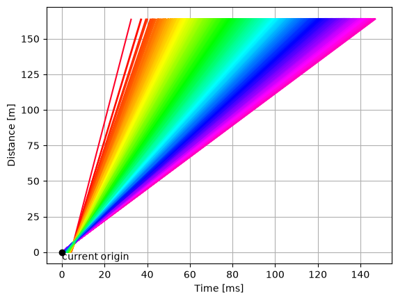
As the figure above illustrates, the current time-of-flight computation (tof = toa - time_origin) assumes that all neutrons were born at \(t = 0\) (black dot).

This is clearly not the case from looking at the neutron tracks.

Exercise: find a new origin

• Inspect the time-distance diagram and try to find a point which would be a better representation of a common origin for all tracks.

• Set the origin as coordinates on the original data (hint: you will need to update the source_position and time_origin coordinates).

• Compute wavelength/d-spacing again.

Solution:

Show code cell content

Hide code cell content

better = sample_si.copy(deep=False)

# Read off the plot that the lines cross as they go through the chopper:
# time=5.53, distance=6.5 (approximately)
better.coords['source_position'] = sc.vector([0, 0, 6.5], unit='m')
better.coords['time_origin'] = sc.scalar(5.53, unit='ms').to(unit='s')

better_dspacing = better.transform_coords("dspacing", graph=graph)
better_dspacing

scipp.DataArray (139.14 MB)

• Dimensions:
  • events: 868421
• Coordinates: (20)
  • L1
    ()
    float64
    m
    154.1365294631786

    Values:
    array(154.13652946)

  • L2
    (events)
    float64
    m
    3.558, 3.502, ..., 3.534, 3.505

    Values:
    array([3.55758433, 3.50180757, 3.50501872, ..., 3.52422421, 3.5337878 ,
           3.50501872], shape=(868421,))

  • Ltotal
    (events)
    float64
    m
    157.694, 157.638, ..., 157.670, 157.642

    Values:
    array([157.69411379, 157.63833703, 157.64154819, ..., 157.66075367,
           157.67031727, 157.64154819], shape=(868421,))

  • dspacing
    (events)
    float64
    Å
    1.920, 1.637, ..., 1.922, 1.635

    Values:
    array([1.91994202, 1.6365862 , 3.1338877 , ..., 1.36001117, 1.92249656,
           1.6348507 ], shape=(868421,))

  • incident_beam
    ()
    vector3
    m
    [ 1.44691967 0. 154.12973801]

    Values:
    array([  1.44691967,   0.        , 154.12973801])

  • position
    (events)
    vector3
    m
    [ 4.73058934 -0.6375 159.41832831], [4.93729531e+00 1.12500000e-01 1.60370358e+02], ..., [ -2.03227752 -0.4875 161.01077207], [ -1.95277758 0.1875 159.79783738]

    Values:
    array([[ 4.73058934e+00, -6.37500000e-01,  1.59418328e+02],
           [ 4.93729531e+00,  1.12500000e-01,  1.60370358e+02],
           [ 3.93256848e+00,  1.87500000e-01,  1.63093790e+02],
           ...,
           [-6.47216436e-01, -4.12500000e-01,  1.57825350e+02],
           [-2.03227752e+00, -4.87500000e-01,  1.61010772e+02],
           [-1.95277758e+00,  1.87500000e-01,  1.59797837e+02]],
          shape=(868421, 3))

  • sample_position
    ()
    vector3
    m
    [ 1.44691967 0. 160.62973801]

    Values:
    array([  1.44691967,   0.        , 160.62973801])

  • scattered_beam
    (events)
    vector3
    m
    [ 3.28366968 -0.6375 -1.2114097 ], [ 3.49037565 0.1125 -0.25937972], ..., [-3.47919718 -0.4875 0.38103406], [-3.39969724 0.1875 -0.83190062]

    Values:
    array([[ 3.28366968, -0.6375    , -1.2114097 ],
           [ 3.49037565,  0.1125    , -0.25937972],
           [ 2.48564881,  0.1875    ,  2.46405154],
           ...,
           [-2.0941361 , -0.4125    , -2.80438834],
           [-3.47919718, -0.4875    ,  0.38103406],
           [-3.39969724,  0.1875    , -0.83190062]], shape=(868421, 3))

  • sim_source_time
    (events)
    float64
    s
    7.857e-05, 0.002, ..., 0.001, 0.001

    Values:
    array([7.85670313e-05, 1.69307755e-03, 1.69307755e-03, ...,
           1.46205143e-03, 1.46205143e-03, 1.46205143e-03], shape=(868421,))

  • sim_speed
    (events)
    float64
    m/s
    1259.946, 1657.737, ..., 1535.014, 1535.014

    Values:
    array([1259.9463418 , 1657.73712122, 1657.73712122, ..., 1535.01388466,
           1535.01388466, 1535.01388466], shape=(868421,))

  • sim_wavelength
    (events)
    float64
    Å
    3.140, 2.386, ..., 2.577, 2.577

    Values:
    array([3.13984325, 2.38640612, 2.38640612, ..., 2.57719755, 2.57719755,
           2.57719755], shape=(868421,))

  • source_position
    ()
    vector3
    m
    [0. 0. 6.5]

    Values:
    array([0. , 0. , 6.5])

  • time_origin
    ()
    float64
    s
    0.00553

    Values:
    array(0.00553)

  • toa
    (events)
    float64
    s
    0.130, 0.101, ..., 0.108, 0.108

    Values:
    array([0.13043615, 0.10069373, 0.10069623, ..., 0.1084057 , 0.1084108 ,
           0.10838834], shape=(868421,))

  • tof
    (events)
    float64
    s
    0.125, 0.095, ..., 0.103, 0.103

    Values:
    array([0.12490615, 0.09516373, 0.09516623, ..., 0.1028757 , 0.1028808 ,
           0.10285834], shape=(868421,))

  • two_theta
    (events)
    float64
    rad
    1.909, 1.636, ..., 1.472, 1.820

    Values:
    array([1.90904466, 1.63555193, 0.78181936, ..., 2.50024339, 1.472057  ,
           1.81980186], shape=(868421,))

  • wavelength
    (events)
    float64
    Å
    3.133, 2.388, ..., 2.581, 2.581

    Values:
    array([3.13349029, 2.3881941 , 2.38820814, ..., 2.58136373, 2.58133526,
           2.58124265], shape=(868421,))

  • x
    (events)
    float64
    m
    4.731, 4.937, ..., -2.032, -1.953

    Values:
    array([ 4.73058934,  4.93729531,  3.93256848, ..., -0.64721644,
           -2.03227752, -1.95277758], shape=(868421,))

  • y
    (events)
    float64
    m
    -0.637, 0.113, ..., -0.487, 0.188

    Values:
    array([-0.6375,  0.1125,  0.1875, ..., -0.4125, -0.4875,  0.1875],
          shape=(868421,))

  • z
    (events)
    float64
    m
    159.418, 160.370, ..., 161.011, 159.798

    Values:
    array([159.41832831, 160.37035829, 163.09378954, ..., 157.82534966,
           161.01077207, 159.79783738], shape=(868421,))

• Data: (1)
  • (events)
    float64
    counts
    0.693, 1.351e-27, ..., 7.612e-11, 6.337e-11

    σ = 0.693, 1.351e-27, ..., 7.612e-11, 6.337e-11

    Values:
    array([6.93355652e-01, 1.35069699e-27, 9.19423594e-28, ...,
           2.52357063e-11, 7.61208643e-11, 6.33685313e-11], shape=(868421,))
    
    Variances (σ²):
    array([4.80742060e-01, 1.82438235e-54, 8.45339746e-55, ...,
           6.36840872e-22, 5.79438598e-21, 4.01557076e-21], shape=(868421,))

better_dspacing.hist(two_theta=ntheta, dspacing=dbins).plot(norm='log', vmin=1.0e-3)

pp.plot({'original': si_dspacing_hist.sum('two_theta'),
         'improved': better_dspacing.hist(two_theta=ntheta, dspacing=dbins).sum('two_theta')})

Exercise 3: Process the Vanadium run

We now need to repeat the process (load data, correct time-of-flight, convert to d-spacing) for the Vanadium run.

folder = "../3-mcstas/output_sample_vanadium"

⚠️ If you did not complete the Vanadium simulation yesterday, you can use some pre-prepared data by uncommenting and running the cell below:

# folder = utils.fetch_data("3-mcstas/output_sample_vanadium")

sample_van = utils.load_powder(folder)

Show code cell content

Hide code cell content

# Read off the plot that the lines cross as they go through the chopper:
# time=5.53, distance=6.5 (approximately)
sample_van.coords['source_position'] = sc.vector([0, 0, 6.5], unit='m')
sample_van.coords['time_origin'] = sc.scalar(5.53, unit='ms').to(unit='s')
# Convert to dspacing
van_dspacing = sample_van.transform_coords("dspacing", graph=graph)

van_dspacing.hist(two_theta=ntheta, dspacing=dbins).plot(norm='log', vmin=1.0e-3)

Normalize by Vanadium

The next step in our data reduction is to normalize our sample signal by the Vanadium counts.

Vanadium is an almost perfect incoherent scatterer (scatters equally in all directions) and the signal from that run can be used to correct for difference in detector exposure and sensitivity.

Performing accurate normalization is a complex subject, but in our simple idealised set-up, it basically boils down to a simple division operation.

We first histogram the sample and vanadium data using the same binning for both:

num = better_dspacing.hist(two_theta=ntheta, dspacing=dbins)
den = van_dspacing.hist(two_theta=num.coords['two_theta'], dspacing=dbins)

For best results, it is common practice to smooth the Vanadium signal before using it for normalization, to remove any noise that mostly comes from collection statistics rather than detector efficiency.

We thus smooth the Vandium histogram using a simple Gaussian filter. We will normalize the signal as a 1D histogram, so the data is first summed over the two_theta dimension. In Scipp, because of the physical units, we can define a physical kernel width as opposed to having to determine how many neighbours are necessary for good smoothing.

# Smooth the Vanadium run 
from scipp.scipy.ndimage import gaussian_filter

smooth_vana = gaussian_filter(
    sc.values(den.sum('two_theta')),
    sigma=sc.scalar(0.03, unit='angstrom')
)

pp.plot({'orig': den.sum('two_theta'), 
         'smooth': smooth_vana}, 
        title='Vanadium - smoothed')

Exercise 4: perform the normalization

Finally, we divide the sample histogram num (summed over two_theta) by the smoothed Vanadium.

Show code cell content

Hide code cell content

normed = (num.sum('two_theta') / smooth_vana)

normed.plot()

You can compare to the plot above (before normalization) and see that the relative intensities of the Si peaks have changed.

Save to disk

We now need to save our reduced normalized data to a file, that will then be used by the analysis software in the next chapter.

For this, we use a small helper function:

utils.save_xye("reduced_Si.xye",
               event_data=better_dspacing,  # Needed for saving metadata required for analysis
               normalized_histogram=normed)

Exercise 5: Process and normalize main sample: LBCO

Repeat the process for the LBCO sample:

• load data

• correct time-of-flight

• convert to d-spacing

• normalize by Vanadium

• save to disk

folder = "../3-mcstas/output_sample_LBCO"

⚠️ If you did not complete the Si simulation yesterday, you can use some pre-prepared data by uncommenting and running the cell below:

# folder = utils.fetch_data("3-mcstas/output_sample_LBCO")

Show code cell content

Hide code cell content

lbco = utils.load_powder(folder)

# Read off the plot that the lines cross as they go through the chopper:
# time=5.53, distance=6.5 (approximately)
lbco.coords['source_position'] = sc.vector([0, 0, 6.5], unit='m')
lbco.coords['time_origin'] = sc.scalar(5.53, unit='ms').to(unit='s')

lbco_dspacing = lbco.transform_coords("dspacing", graph=graph)
lbco_dspacing.hist(two_theta=ntheta, dspacing=dbins).plot(norm='log', vmin=1.0e-3)

# Normalize
lbco_num = lbco_dspacing.hist(two_theta=den.coords['two_theta'], dspacing=dbins)

lbco_normed = (lbco_num.sum('two_theta') / smooth_vana)

lbco_normed.plot()

Show code cell content

Hide code cell content

# Save to disk
utils.save_xye("reduced_LBCO.xye",
               event_data=lbco_dspacing,  # Needed for saving metadata required for analysis
               normalized_histogram=lbco_normed)