Making more complex models in EasyScience#
On top of interfacing with various 3rd party minimization libraries, easyscience also implements functionality to ease the creation of more complex models.
In this exercise we will explore bounded parameters as well as dependent parameters, which are two ways to constrict model parameters to certain ranges/values.
🛠️ Import Library#
Just like before we start by importing the easyscience library and other supporting libraries.
import numpy as np
import matplotlib.pyplot as plt
from easyscience import global_object
We disable the legacy warning again.
global_object.log.getLogger('legacy').setLevel('ERROR') # suppress warnings from legacy code in this notebook
And import easyscience
import easyscience as es
📘 Introduction: Bounded Parameters#
In the previous notebook, model parameters were free to take any values between \(-\infty\) and \(\infty\).
When these parameters reflect real physical properties, this often does not make sense. You cannot have a negative temperature in Kelvin, or a negative area. An electron occupation can only be between 0 and 1, etc.
To account for this, it is possible to set minimum and maximum values for parameters, i.e. to bound them. These parameter bounds are then respected when the likelihood is maximized.
We use the same data as in the previous notebook.
import numpy as np

np.random.seed(123)

a_true = -0.9594
b_true = 7.294
c_true = 3.102

N = 25
x = np.linspace(0, 10, N)
yerr = 1 + 1 * np.random.rand(N)
y = a_true * x ** 2 + b_true * x + c_true
y += np.abs(y) * 0.1 * np.random.randn(N)
Information about bounds can be included in easyscience parameters as min and max values.
a = es.Parameter(name='a', value=-0.9, fixed=False, min=-5.0, max=0.5)
b = es.Parameter(name='b', value=6.9, fixed=False, min=0, max=7)
c = es.Parameter(name='c', value=3.0, fixed=False, min=-20, max=50)
We can then perform the analysis in the same fashion as previously, however, this time the bounds will be respected.
def math_model(x, *args, **kwargs):
    return a.value * x ** 2 + b.value * x + c.value

quad = es.ObjBase(name='quad', a=a, b=b, c=c)
fitter = es.Fitter(quad, math_model)

results = fitter.fit(x=x, y=y, weights=yerr)

a, b, c, results
(<Parameter 'a': -0.9127 ± 0.0373, bounds=[-5.0:0.5]>,
 <Parameter 'b': 7.0000 ± 0.2990, bounds=[0.0:7.0]>,
 <Parameter 'c': 2.2129 ± 0.8501, bounds=[-20.0:50.0]>,
 FitResults(success=True
   n_pars=3, n_points=25
   chi2=117.5, reduced_chi2=5.339
   n_evaluations=26
   iterations=26
   minimizer=LMFit
   message='Fit succeeded.'
   parameters={pParameter_0=-0.9127, pParameter_1=7, pParameter_2=2.213}
 ))
Note
Notice that the “b” parameter hit its upper bound and was not allowed to go above that to reach it’s true value of 7.294.
📘 Introduction: Parameter Arithmetics#
easyscience parameters can also have units and uncertainties (the uncertainty usually get’s filled in after fitting).
These fields become relevant when you want to do post-processing of your model parameters.
For example, you might have fitted the sizes of a reflectometry layer model to your data, and is now interested in the total volume of your sample (according to your fit).
Say we have 3 layers with 3 different thicknesses, but all layers share width and length. First, we create these 5 parameters.
layer_1 = es.Parameter(name='layer_1', value=1.37, variance=0.32, unit='cm', min=0.0, max=10)
layer_2 = es.Parameter(name='layer_2', value=8.35, variance=4.68, unit='mm', min=0.0, max=20)
layer_3 = es.Parameter(name='layer_3', value=0.89, variance=0.02, unit='cm', min=0.0, max=1.0)
width = es.Parameter(name='width', value=20.31, variance=2.46, unit='cm', min=15, max=25)
length = es.Parameter(name='length', value=19.86, variance=1.76, unit='cm', min=15, max=25)
We have here simulated the resultant parameters after a fit hence the uncertainties given by the “variance” argument.
Notice that the thicknesses have min=0.0 while the width and lengths have min=15. This is simulating that the real physical sample might be visibly larger than 15cm (and smaller than 25cm) but the thicknesses of the individual layers cannot be discnered by the naked eye, yet we know a thicnkess can’t be negative. Note also that one of the thickness parameters have a different unit than the rest.
Now, to calculate the total thickness of the sample, we can simply add up our parameters:
layer_1 + layer_2 + layer_3
<Parameter 'Parameter_9': 3.0950 ± 0.6219 cm, bounds=[0.0:13.0]>
Notice that the output is a new parameter whose value is the values added up correctly, with their units taken into consideration.
The uncertainties are also propagated correctly in these arithmetic operations, using uncertainty propagation, and the bounds are also added up, hence the maximum of 13 cm.
When adding/subtracting parameters with different yet compatible units, the 2nd operand is converted to the unit of the first operand. Notice the difference here.
layer_2 + layer_1 + layer_3
<Parameter 'Parameter_11': 30.9500 ± 6.2193 mm, bounds=[0.0:130.0]>
Because the first operand is the parameter with a unit of “mm”, the entire result, including uncertainty and bounds gets converted to the unit of “mm”.
You cannot add/subtract parameters with incompatible units i.e. parameters of different dimensions, this includes bare numbers.
test_parameter = es.Parameter(name='test', value=55, unit='s')
layer_1 + test_parameter
layer_1 + 20
You can however add/subtract dimensionless parameters with simple numbers.
temporary = es.Parameter(name='unitless', value=20, variance=5, min=-4, max=66)
temporary + 34
<Parameter 'Parameter_13': 54.0000 ± 2.2361, bounds=[30.0:100.0]>
Parameters don’t need to have uncertainties and bounds to be used in arithmetic operations. The existing bounds and uncertainties will still be propagated correctly.
test_parameter = es.Parameter(name='test', value=1e8, unit='angstrom')
test_parameter + layer_1
<Parameter 'Parameter_15': 2.370e+08 ± 5.657e+07 Å, bounds=[-inf:inf]>
You can also do multiplication and division of parameters, so returning to our example, we could calculate the volume of the sample by simply multiplying the total thickness with the width and length.
(layer_1 + layer_2 + layer_3)*width*length
<Parameter 'Parameter_19': 1248.3887 ± 281.3887 mL, bounds=[0.0:8125.0]>
Notice that the unit now correctly gets converted into a unit of the correct dimensionality, here a volume. You can change the desired unit to another unit of the same dimension using the “convert_unit” method on the output parameter.
output = ((layer_1 + layer_2 + layer_3)*width*length)
output.convert_unit('L')
output
<Parameter 'Parameter_23': 1.2484 ± 0.2814 L, bounds=[0.0:8.125000000000002]>
It is also possible to multiply/divide by pure numbers, which also impacts uncertainties and bounds.
output*3.14
<Parameter 'Parameter_24': 3.9199 ± 0.8836 L, bounds=[0.0:25.512500000000006]>
Note
Supported operations currently only include addition, subtraction, multiplication, division, negation and exponentiation.
There are plans to extend this list to geometric functions in the future.
Division by a parameter with a value of zero will result in a ZeroDivisionError.
📘 Introduction: Dependent Parameters#
Sometimes models have more parameters than degrees of freedom. Take for example a cube with sides a, b and c.
You might let all the parameters be free to vary, but you might also require that they all be equal. In this case you have 3 parameters but only 1 degree of freedom.
You could also have a specific relation between the cubes sides, a being twice the size of b or c being equal to a plus b. Such relations can be made in easyscience using dependent parameters.
To showcase this, first we create the 3 side parameters.
a = es.Parameter(name='a', value=5, unit='m', min=0.0)
b = es.Parameter(name='b', value=10, unit='m', min=0.0)
c = es.Parameter(name='c', value=2, unit='m', min=0.0)
Say we want the side c to be equal to a plus b, we can use the parameter arithmetics we just learned to define the relationship using the make_dependent_on method.
c.make_dependent_on(
    dependency_expression = 'side_a + side_b',
    dependency_map = {'side_a':a, 'side_b':b}
)
c
<Parameter 'c': 15.0000 m, bounds=[0.0:inf]>
The “dependency_expression” is the expression determining the value of the dependent parameter. The “dependency_map” tells the dependent parameter, what parameters the names in the “dependency_expressions” corresponds to.
The parameter c is now a dependent parameter, it’s value cannot be changed manually or by the fitter, instead it updates automatically when its dependencies’ values are updates.
a.value = 2
c
<Parameter 'c': 12.0000 m, bounds=[0.0:inf]>
The dependent parameter also gets updated on uncertainty changes, bound changes or unit changes.
a.convert_unit('cm')
c
<Parameter 'c': 1200.0000 cm, bounds=[0.0:inf]>
The “dependency_expression” can be just another parameter, to constrain the dependent parameter to be equal to the other parameter, or it can be any valid arithmetic operation on parameters.
To make a parameter independent again, to free it up for varying during fits, use the “make_independent” method. It will keep its current values/units etc. but they are now free to be changed.
c.make_independent()
print(c)
c.max=5000
print(c)
<Parameter 'c': 1200.0000 cm, bounds=[0.0:inf]>
<Parameter 'c': 1200.0000 cm, bounds=[0.0:5000.0]>
If you know beforehand that a parameter should be dependent, there is no need to first create it and then make it dependent, you can use the convenience function “from_dependency” to directly create dependent parameters.
volume = es.Parameter.from_dependency(
    name='volume',
    dependency_expression='a*b*c',
    dependency_map={'a':a, 'b':b, 'c':c}
)
print(volume)
c.value = 2000  # Its current unit is cm.
print(volume)
<Parameter 'volume': 2.400e+05 L, bounds=[0.0:inf]>
<Parameter 'volume': 4.000e+05 L, bounds=[0.0:inf]>
It is also possible to do simple logic dependencies, and dependencies of dependencies.
package_volume = es.Parameter.from_dependency(
    name='package_volume',
    dependency_expression='1.5*v if v.value < 2.0e5 else 2*v',
    dependency_map = {'v' : volume}
)
print(volume)
print(package_volume)
c.value = 900
print(volume)
print(package_volume)
<Parameter 'volume': 4.000e+05 L, bounds=[0.0:inf]>
<Parameter 'package_volume': 8.000e+05 L, bounds=[0.0:inf]>
<Parameter 'volume': 1.800e+05 L, bounds=[0.0:inf]>
<Parameter 'package_volume': 2.700e+05 L, bounds=[0.0:inf]>
Dependent parameters have many uses, such as enforcing symmetry constraints or value relations, but dependent parameters can also simply reflect a post-analysis property which you wish to inspect while manually (or automatically) changing the model parameters.
💪 Exercise: Gaussian and Lorentzian mixture#
Create a normalized Gaussian model as well as a normalized Lorentzian model. The normalized Gaussian model is simply the Gaussian model from the previous notebook with a specific amplitude.
Then create a mixture model, adding both models together in fractions, ensuring that their fractions add up to 1 using what you just learned.
The normalized Lorentzian model takes the following form:
Where \(A\) is the amplitude of the Lorentzian, \(x_0\) is its mean/center point and \(\gamma\) is its width (HWHM).
The normalized Gaussian model takes the following form:
Where \(A\) is the amplitude of the Gaussian, \(\mu\) is the mean/center point of the Gaussian and \(\sigma\) is its width/standard deviation.
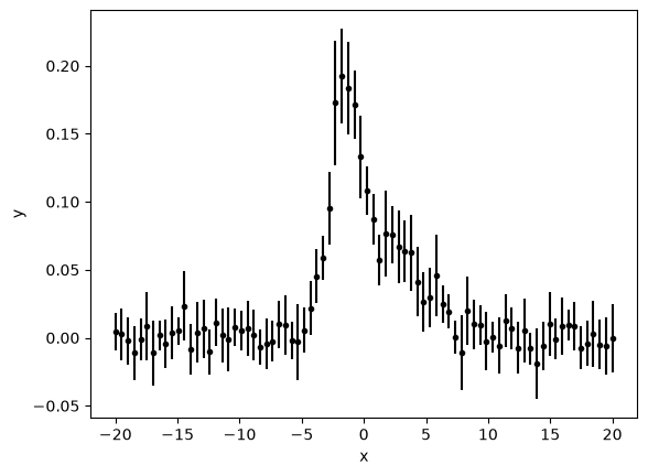
First we manufacture the data to be fitted.
np.random.seed(1337)

N = 80

x = np.linspace(-20, 20, N)

from scipy.stats import Normal
mu = (np.random.rand(1)-0.5)*6
sigma = np.random.rand(1)*2+1
gauss = Normal(mu=mu, sigma=sigma)
y_gauss = gauss.pdf(x)
yerr_gauss = 0.03 * np.random.rand(N) + 0.1*y_gauss*np.random.rand(N) + 0.01 + 0.05*y_gauss
y_gauss += 2*(np.random.rand(N)-0.5)*yerr_gauss

np.random.seed(314)
from scipy.stats import cauchy
x0 = (np.random.rand(1)-0.5)*6
gamma = np.random.rand(1)*2+1
y_lorentz = cauchy.pdf(x, loc=x0, scale=gamma)
yerr_lorentz = 0.01 * np.random.rand(N) + 0.05*y_lorentz*np.random.rand(N) + 0.005 + 0.05*y_lorentz
y_lorentz += 2*(np.random.rand(N)-0.5)*yerr_lorentz

np.random.seed(67)
fraction = np.random.rand(1)
y = fraction*y_gauss + (1-fraction)*y_lorentz
yerr = fraction*yerr_gauss + (1-fraction)*yerr_lorentz
plt.errorbar(x, y, yerr, marker='.', ls='', color='k')
plt.xlabel('x')
plt.ylabel('y')
plt.show()
🧩 Exercise 1: Create the Gaussian model#
Create the 3 easyscience Parameters corresponding to the 3 parameters of the Gaussian model: the Amplitude \(A\), the Mean \(\mu\) and the width \(\sigma\) and create the python function, like in the previous notebook.
Solution:
🧩 Exercise 2: Normalize the Gaussian model#
Since Numpy cannot be used in dependency expressions, we first create a static easyscience parameter called a DescriptorNumber and assign it the value of np.pi.
DescriptorNumbers are used for numerical or physical constants, they cannot be used in fitting and hence don’t have bounds.
They can however still have uncertanties and units (if assigned to them). More importantly, they can be used in dependency expressions if added to the dependency_map.
pi = es.DescriptorNumber(name='pi', value=np.pi)
Now, make the amplitude of the Gaussian model a dependent parameter according to the equation above to ensure that it is normalized.
Hint:
Remember that raising something to the power of 0.5 is equivalent to taking the square root.
Hint:
Don’t forget to set your parenthesis right, that exponentiation in Python is done with 2 stars: x**2 is \(x^2\) and call parameter.value to access parameter values in the function
Solution:
🧩 Exercise 3: Create the Lorentzian model#
Create the 3 easyscience Parameters corresponding to the 3 parameters of the Lorentzian model: the Amplitude \(A\), the Mean \(x_0\) and the width \(\gamma\) and create the python function
Solution:
🧩 Exercise 4: Normalize the Lorentzian model#
Just like with the Gaussian model, make the Lorentzian amplitude a dependent parameter to ensure that the lorentzian is normalized.
Solution:
🧩 Exercise 5: Create the mix fraction parameters#
Create 2 easyscience Parameters, the first should be bounded to the interval [0:1] and the other should be a dependent parameter with expression 1 minus the other parameter.
This setup allows both parameters to range between 0 and 1, corresponding to 0 and 100% mixing fraction, and ensures that they add up to 100%.
Hint:
The syntax for setting bounds on a parameter (min/max) is shown higher up in this notebook.
Hint:
Don’t forget that parameters with units can’t be added/subtracted with real numbers. Ensure that your fraction parameter is unitless by not passing the unit keyword argument
Solution:
🧩 Exercise 6: Create the mixed model#
Use the fraction parameters defined just now, and the gaussian and lorentzian model to define a new python function reflecting the mixture model.
Hint:
Don’t forget that you can call your previously defined python functions within the new python function.
Solution:
🚀 Exercise 7: Setup and perform the fit#
Create the ObjBase to hold the Parameters and use your newly defined mixture model when setting up your Fitter.
Tune the Fitters configuration if you desire and perform the fit.
Hint:
Check the previous notebook if you forgot how to setup and execute the fitting procedure.
Hint:
The ObjBase should hold all parameters to be fitted, i.e. both the Gaussian and Lorentzian parameters as well as the mixture parameters.
Solution:
(<Parameter 'mean': -1.4332 ± 0.0600, bounds=[-inf:inf]>,
 <Parameter 'width': 1.2042 ± 0.0576, bounds=[-inf:inf]>,
 <Parameter 'mean': 2.2760 ± 0.1470, bounds=[-inf:inf]>,
 <Parameter 'width': 2.3748 ± 0.2023, bounds=[-inf:inf]>,
 <Parameter 'fraction': 0.5146 ± 0.0216, bounds=[0.0:1.0]>,
 <Parameter 'fraction': 0.4854 ± 0.0216, bounds=[0.0:1.0]>,
 FitResults(success=True
   n_pars=5, n_points=80
   chi2=14.42, reduced_chi2=0.1922
   n_evaluations=56
   iterations=56
   minimizer=LMFit
   message='Fit succeeded.'
   parameters={pParameter_37=-1.433, pParameter_38=1.204, pParameter_44=2.276, pParameter_45=2.375, pParameter_50=0.5146}
 ))
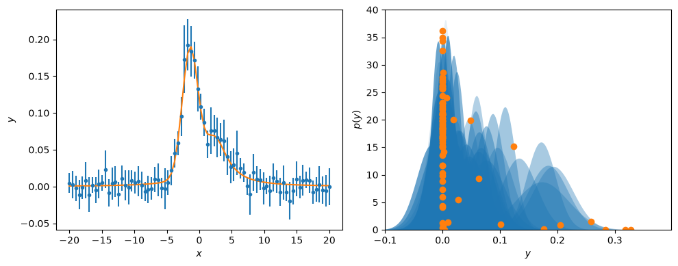
Don’t forget to inspect your results, your fitted values for the parameters, the goodness of the fit and the visual comparison of how well the model fits the data.
from scipy.stats import norm

fig, ax = plt.subplots(1, 2, figsize=(10, 4))

ax[0].errorbar(x, y, yerr, marker='.', ls='', color='C0')
ax[0].plot(x, mixture(x), '-', color='C1')
ax[0].set_xlabel('$x$')
ax[0].set_ylabel('$y$')

y_range = np.arange(-0.1, 0.4, 0.002)
for i, yy in enumerate(y):
    ax[1].fill_between(y_range, norm(yy, yerr[i]).pdf(y_range), color='C0', alpha=0.01 * (i + 1), lw=0)
    ax[1].plot(gaussian_model(x[i]), norm(yy, yerr[i]).pdf(gaussian_model(x[i])), 'C1o')
ax[1].set_xlim(y_range.min(), y_range.max())
ax[1].set_ylim(0, None)
ax[1].set_xlabel('$y$')
ax[1].set_ylabel('$p(y)$')
plt.tight_layout()
plt.show()
You will now move on to try out these methods with your own neutron data and more complex and technique-specific models.