SANS analysis#
Part I: Fitting data#
Previously, some small angle neutron scattering (SANS) data has been simulated and reduced, and can now be analysed.
Before the analysis can begin, it is necessary to load the experimental data and check that it looks reasonable.
The data can be loaded with np.loadtxt as the data has been stored in a simple space-separated column file.
import numpy as np
import utils
from sans_fitter import SANSFitter
filename = "../4-reduction/sans_iofq.dat"
q, i, di = utils.load(filename)
With the data read in, we can produce a quick plot simply using matplotlib.
import matplotlib.pyplot as plt

fig, ax = plt.subplots()
ax.errorbar(q, i, di, fmt=".")
ax.set(yscale="log", xlabel="$q$/Å^-1", ylabel="I(q)")
plt.show()
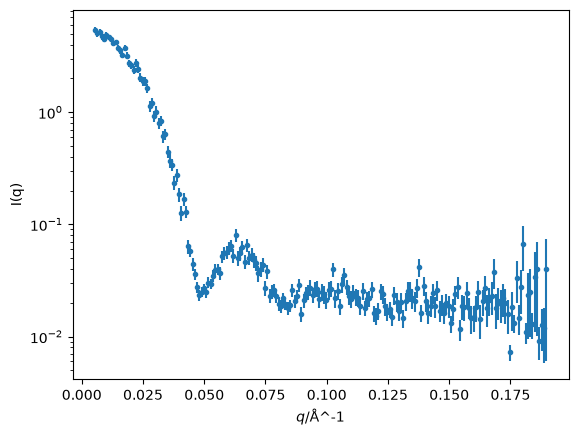
We now want to consider the mathematical model to be used in the analysis. There are SANS models for myriad systems, see the models in SasView. Initially, we will assume that our data has arisen from a spherical scattering object.
The mathematical model for a sphere is:
where \(\text{scale}\) is a scale factor, \(V\) is the volume of the sphere, \(\Delta \rho\) is the difference between the solvent and particle scattering length density (\(\rho_{solvent}\) - \(\rho_{scatterer}\)), \(r\) is the radius of the sphere, a uniform background is added, and finally \(q\) is the q-vector that the intensity is being calculated for.
Exercise 1: simplify the expression#
The mathematical model described in Eqn. (3) has five parameters. What simple mathematical simplification can be performed to reduce this to four?
Solution:
Exercise 2: write a function that computes for the form factor of a sphere#
Four parameters is a suitable number for modelling. Therefore, we should write a function that implements your reduced dimensionality version of Eqn. (3).
Exercise 3: create fitting parameters#
sans-fitter provides a notebook-based backend for interaction with sasmodels, the most comprehensive community library of fitting functions for small-angle scattering data (used in the popular SasView GUI application).
All of the functions here are 100% equivalent to working in the SasView GUI : You could even complete these tasks using the GUI, if you are more comfortable. However, we encourage you to try the Jupyter notebook approach below for these exercises!
We imported sans-fitter at the top of the notebook. Now, one can create the fitter, load the SANS dataset above, and then fetch the sphere model and its default parameters:
fitter = SANSFitter()

fitter.load_data(filename)
fitter.set_model("sphere")
fitter.get_params()
✓ Loaded data from ../4-reduction/sans_iofq.dat
  Q range: 0.0055 to 0.1895 Å⁻¹
  Data points: 200
  Error (dI) column: yes
  Resolution (dQ) column: no
✓ Model 'sphere' loaded successfully
  Available parameters: 5

================================================================================
Model: sphere
================================================================================
Parameter            Value        Min          Max          Vary
--------------------------------------------------------------------------------
sld                  1            0            10           ✗
sld_solvent          6            0            60           ✗
radius               50           0            500          ✗
scale                1            0            inf          ✗
background           0            0            inf          ✗
================================================================================
Knowing the parameters, we can proceed to assign sensible initial values, uniform prior distributions, define whether the parameters are to be fitted or fixed, and then confirm that we have passed these correctly.
You will note that sans-fitter identifies the presence, or absence, of experimental intensity error (dI) and resolution (dQ) in the provided data file. Accounting for aspects such as these complicates the implementation of fitting, beyond just applying a simple sphere form factor, like we derived earlier.
fitter.set_param("sld", value=3, min=1, max=30, vary=False)
fitter.set_param("sld_solvent", value=6, min=1, max=30, vary=False)

fitter.set_param("radius", value=80, min=10, max=300, vary=True)
fitter.set_param("scale", value=1.4e-7, min=0, max=1, vary=True)
fitter.set_param("background", value=0.1, min=0, max=1, vary=True)

fitter.get_params()
================================================================================
Model: sphere
================================================================================
Parameter            Value        Min          Max          Vary
--------------------------------------------------------------------------------
sld                  3            1            30           ✗
sld_solvent          6            1            30           ✗
radius               80           10           300          ✓
scale                1.4e-07      0            1            ✓
background           0.1          0            1            ✓
================================================================================
Exercise 4: fit the data with the sphere function#
Using sans-fitter, we can now fit the data and obtain maximum likelihood estimates for the varied parameters of the model.
We can start by using the BUMPS engine with the Nelder-Mead simplex method.
result = fitter.fit(engine="bumps", method="amoeba")
fitter.plot_results(show_residuals=True, log_scale=True)
Initial χ² = 378.8669
Fitting with BUMPS (method: amoeba)...

✓ Fit completed!
Final χ² = 12.4202

Fitted parameters:
  background: 0.01916(31)
  radius: 142.46(59)
  scale: 0.000740(11)
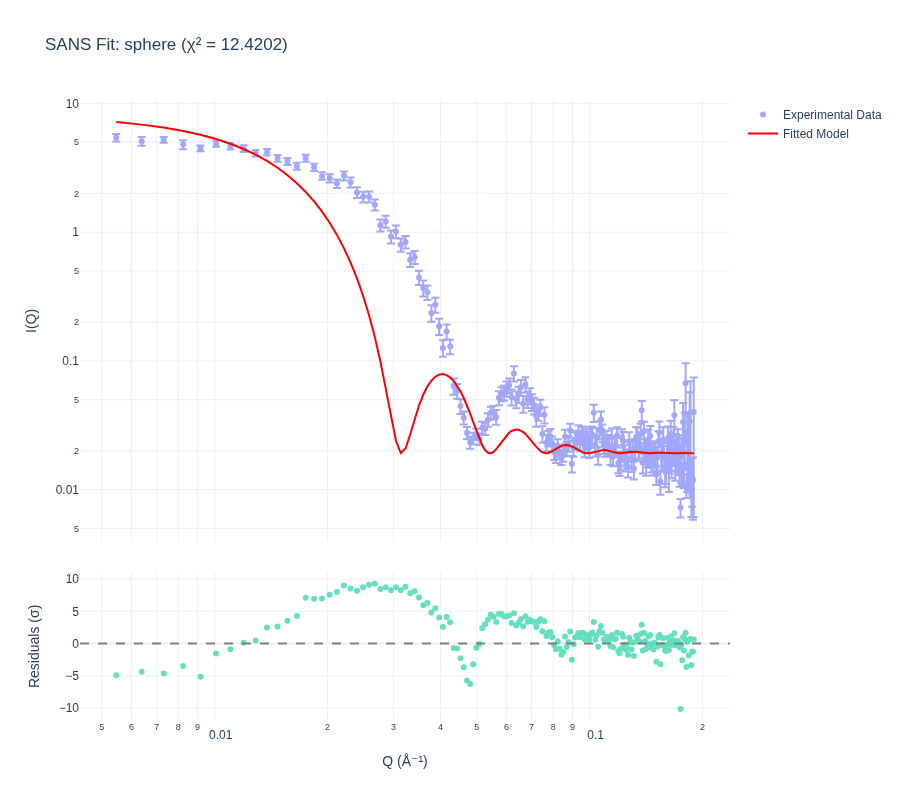
Does the fit look sensible and is the model appropriate?
Are there any ambiguities– are the residuals fine? Could the model be improved?
Exercise 5: fit the data to an ellipsoid model#
In the same way as you have now learned, set the model and find the fitting parameters. Set them to sensible initial values, decide on reasonable ranges, and whether they should be free for the algorithm to optimise, or fixed.
Solution:
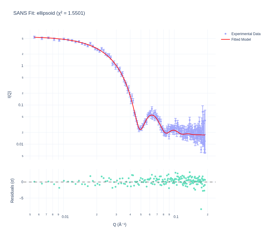
How do the models and their outputs compare?
What is the most appropriate description of the data?
Once you are happy with these fits, continue to Part II: priors and statistics, where we revisit the same dataset using Bayesian methods to obtain full posterior distributions for the model parameters, rather than single best-fit values.