Bayesian analysis of SANS data#
SANS analysis part II: priors and statistics#
You have now simulated, reduced, and carried out routine analysis of your SANS data.
In this notebook, we begin looking at model fitting probabilistically, including prior knowledge about the system or parameters under study in the analysis.
We pick up directly where the previous notebook left off, so we start by loading the same dataset again.
import utils
from sans_fitter import SANSFitter
filename = "../4-reduction/sans_iofq.dat"
Starting with the same dataset, set a sphere model and fetch the parameters, as before.
fitter = SANSFitter()
fitter.load_data(filename)
fitter.set_model("sphere")
fitter.get_params()
✓ Loaded data from ../4-reduction/sans_iofq.dat
  Q range: 0.0055 to 0.1895 Å⁻¹
  Data points: 200
  Error (dI) column: yes
  Resolution (dQ) column: no
✓ Model 'sphere' loaded successfully
  Available parameters: 5

================================================================================
Model: sphere
================================================================================
Parameter            Value        Min          Max          Vary
--------------------------------------------------------------------------------
sld                  1            0            10           ✗
sld_solvent          6            0            60           ✗
radius               50           0            500          ✗
scale                1            0            inf          ✗
background           0            0            inf          ✗
================================================================================
By default, some parameters are set but nothing is allowed to vary. Obviously, this will constrain our fitting algorithm excessively.
In the previous notebook, we included prior knowledge in the analysis through the use of bounded parameters.
Bounded parameters cannot have values less than some lower bound (Min) or greater than some upper bound (Max), as the probability of the parameters having these values is zero.
For example, if the parameter b from a quadratic model has bounds of 0 and 10, then there is an equal probability that the value of b can be anything in between 0 and 10, and a probability of 0 outside those bounds, i.e., it has a uniform prior probability distribution.
Exercise 6: Towards Bayesian analysis#
In this exercise we will repeat the sphere fit from Part I, but treat it probabilistically: the bounds we set act as uniform priors, and instead of a single best-fit value we will obtain a posterior probability distribution for each varied parameter.
The exercise proceeds in three steps:
Set sensible initial values and bounds (priors) for the sphere model, choose which parameters should vary, and confirm the input.
Sample the posterior distribution using the
DREAMMarkov chain Monte Carlo algorithm.Inspect the results with a series of diagnostic plots, and consider what they tell you about the parameters and their uncertainties.
Start with step 1, using the same values and bounds as before:
Great: Now the model is set up, let’s introduce some new syntax for \(Bayesian\) analysis using sans-fitter.
SasView, and hence sans-fitter, have a number of optimisation algorithms built-in. One of these is DREAM, a population based algorithm.
DREAM is relatively slow; it follows a differential evolution-like process but sometimes keeps individuals which get worse with the evolution and allows these to progress as a Markov chain which converges on the equilibrium distribution, where the chain draws randomly from the posterior distribution.
Therefore, we can use the DREAM fitting algorithm to determine parameter uncertainties from our fitting process.
More can be read about DREAM in the associated publication, or in the SasView documentation.
We will begin by setting a few parameters: samples (number of points to be drawn from the Markov chain) and burn (number of iterations for the Markov chain to converge to the equilibrium distribution).
To estimate the 68% interval to two digits of precision, at least 1e5 (or 100,000) samples are needed. For the 95% interval, 1e6 (or 1,000,000) samples are needed. 1e4 samples gives a ‘quick-and-dirty’ approximation of the uncertainty.
result = fitter.fit_bayesian(samples=10000, burn=100)
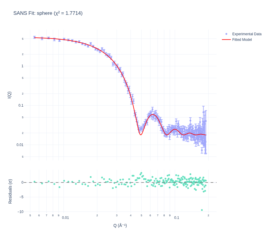
fitter.plot_results(
    show_residuals=True, log_scale=True
)  # Plotting the fit and residuals is the same as before.
Initial χ² = 378.8669
Sampling posterior with BUMPS DREAM (samples=10000, burn=100 generations)...
✓ Fit completed!
Final χ² = 1.7714

Fitted parameters:
  background: 0.01781(30)
  radius: 91.17(29)
  scale: 0.001949(24)

Posterior summary:
Parameter                    Best         Mean       Median          Std                     68% CI                     95% CI
------------------------------------------------------------------------------------------------------------------------------
background              0.0178052    0.0177646    0.0177852  0.000398261     [0.0174775, 0.0180837]      [0.017152, 0.0184109]
radius                    91.1733      91.1285      91.1544      0.51595         [90.8797, 91.4488]         [90.5812, 91.7184]
scale                  0.00194893   0.00194652   0.00194742  2.94842e-05     [0.001924, 0.00197147]   [0.00189876, 0.00199501]

Parameter                 R-hat        ESS
------------------------------------------
background               1.0792        902
radius                   1.2521        866
scale                    1.1710        819
We can now look at the fitting output in detail using a variety of plots:
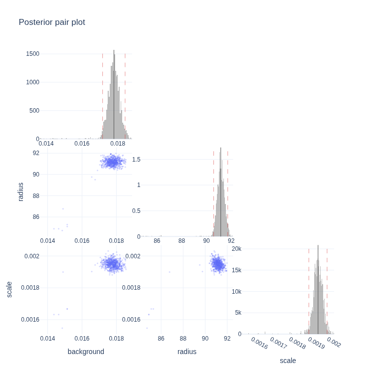
i. A ‘corner’ plot showing a grid of parameter distribution from the Bayesian multi-parameter analysis.
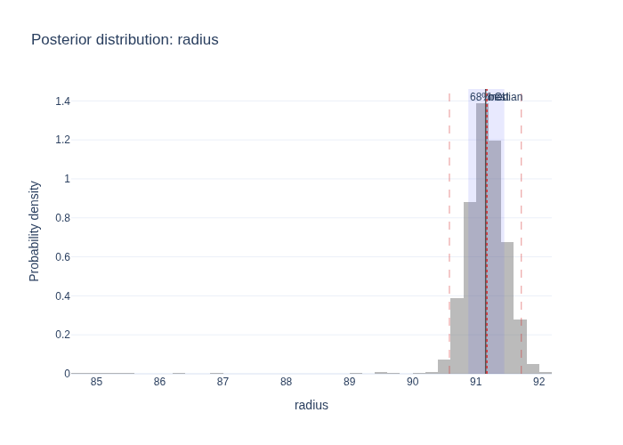
ii. A marginal posterior plot showing the probability distribution for a single, chosen parameter.
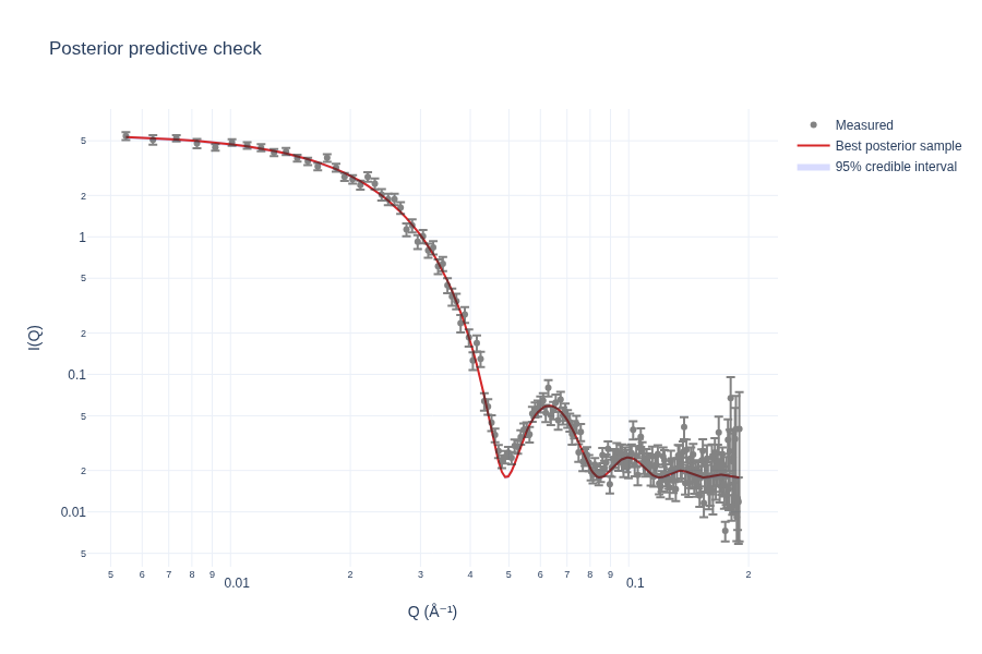
iii. A Bayesian posterior predictive 95% credible band plot, which displays the model’s predicted outcomes over a range of inputs (shaded region may be invisible depending on constraints).
iv. A parameter heatmap giving a colour-coded grid of relationships and statistical dependencies between model parameters estimated from Bayesian inference.
v. The Markov chain Monte Carlo (MCMC) trace which demonstrates how all of the parameters evolved during the fit.
First, the corner plot. Each panel on the diagonal shows the marginal posterior distribution of one varied parameter, while the off-diagonal panels show the pairwise relationships between parameters.
Look out for strongly tilted or curved shapes in the off-diagonal panels: these indicate correlated parameters, which the data cannot constrain independently of one another.
print("\nGenerating posterior pair (corner) plot...")
fitter.plot_posterior_pairs()
Generating posterior pair (corner) plot...
Next, we can single out one parameter of particular interest — here the sphere radius — and inspect its marginal posterior distribution in detail.
Is the distribution symmetric? Roughly Gaussian? The width of this distribution is a direct measure of the uncertainty in the radius.
print("\nGenerating marginal posterior for radius...")
fitter.plot_param_distribution("radius")
Generating marginal posterior for radius...
The posterior predictive plot propagates the parameter uncertainties back into \(I(q)\) space: the shaded band shows the 95% credible interval of the model prediction. If the parameters are tightly constrained, the band may be so narrow that it is barely visible behind the data.
print("\nGenerating posterior predictive band...")
fitter.plot_posterior_predictive(style="band")
Generating posterior predictive band...
The correlation heatmap condenses the off-diagonal information from the corner plot into a single colour-coded matrix of correlation coefficients. Values close to +1 or −1 flag pairs of parameters that the data cannot determine independently.
print("\nGenerating parameter correlation heatmap...")
fitter.plot_param_correlations()
Generating parameter correlation heatmap...
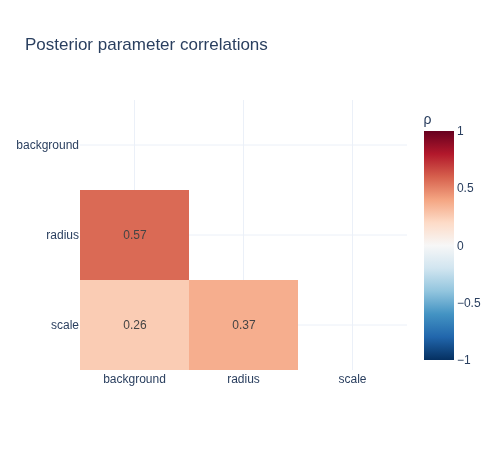
Finally, the MCMC trace shows how each parameter evolved during the sampling. A well-converged chain should look like stationary noise around a constant value; systematic drifts or sudden jumps suggest that more burn iterations or more samples are needed.
print("\nGenerating MCMC trace plot...")
fitter.plot_trace()
Generating MCMC trace plot...
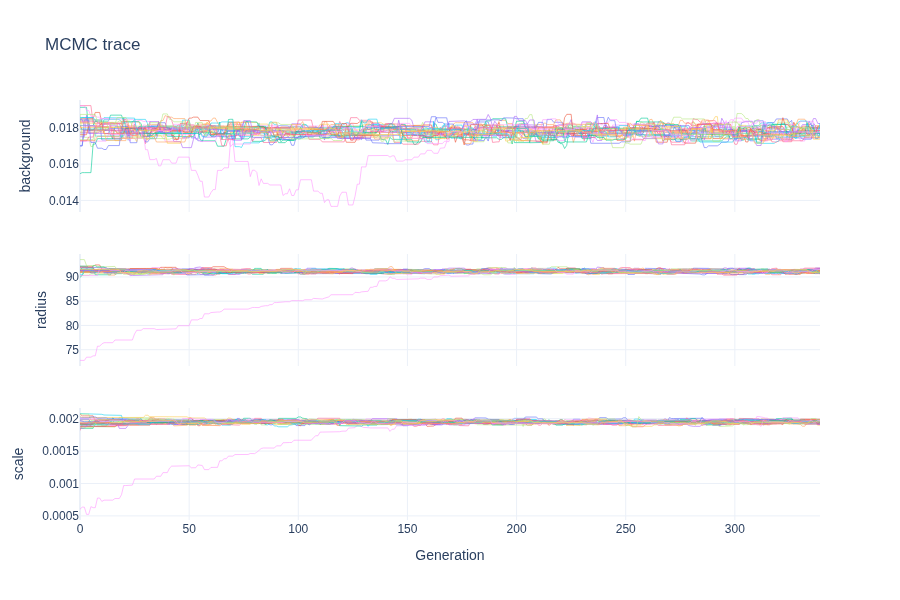
Before moving on, compare these results with the Nelder-Mead fit from the previous notebook:
Are the median parameter values consistent with the maximum likelihood estimates found earlier?
What extra information does the Bayesian analysis provide that a simple optimiser does not?
Finally, an example of how one can access the posterior data and save the fit results:
posterior = fitter.get_posterior()
print("\nSampled parameters:", posterior.labels)
print("Chain shape:", posterior.samples.shape)
print("95% credible intervals:")
for name in posterior.labels:
    low, high = posterior.ci_95[name]
    print(f"  {name}: [{low:.6g}, {high:.6g}]")

# Export the raw chain for external analysis (pandas, corner, arviz, ...)
posterior.save_posterior_csv("posterior_chain.csv")
print("\n✓ Raw posterior chain saved to posterior_chain.csv")

# The saved fit results include the credible intervals in the header
fitter.save_results("bayesian_fit_results.csv")
Sampled parameters: ['background', 'radius', 'scale']
Chain shape: (7530, 3)
95% credible intervals:
  background: [0.017152, 0.0184109]
  radius: [90.5812, 91.7184]
  scale: [0.00189876, 0.00199501]

✓ Raw posterior chain saved to posterior_chain.csv
✓ Results saved to bayesian_fit_results.csv
Exercise 7: Explore models for the data#
You are now armed with knowledge of how to set models, variable and fixed parameters and constraints, and to then fit data with straightforward and more statistically rigorous approaches.
In the previous notebook we explored this dataset using spherical and ellipsoidal fits. Can Bayesian analysis help you to distinguish between candidate models?
In this exercise, you should:
Fetch the list of available models; documentation on these
SasViewmodels can be found here.Pick one, or several, models that could plausibly describe the data.
For each model: create a fitter, set initial values, bounds, and which parameters vary, then run a Bayesian fit with
fit_bayesian.Inspect the fit, residuals, and posterior distributions using the plotting methods from Exercise 6, and decide which model gives the most convincing description of the data.
Further work:
You could also explore the effects of limiting the fitted q-range to see how this limitation affects the statistical distributions:
fitter.set_q_range(qmin=0.1, qmax=0.3)
or try adding a simple structure factor:
fitter.set_structure_factor('hardsphere', radius_effective_mode='link_radius')
from sans_fitter import get_all_models

print(get_all_models())
['adsorbed_layer', 'barbell', 'bcc_paracrystal', 'be_polyelectrolyte', 'binary_hard_sphere', 'broad_peak', 'capped_cylinder', 'core_multi_shell', 'core_shell_bicelle', 'core_shell_bicelle_elliptical', 'core_shell_bicelle_elliptical_belt_rough', 'core_shell_cylinder', 'core_shell_ellipsoid', 'core_shell_parallelepiped', 'core_shell_sphere', 'correlation_length', 'cylinder', 'dab', 'ellipsoid', 'elliptical_cylinder', 'fcc_paracrystal', 'flexible_cylinder', 'flexible_cylinder_elliptical', 'fractal', 'fractal_core_shell', 'fuzzy_sphere', 'gauss_lorentz_gel', 'gaussian_peak', 'gel_fit', 'guinier', 'guinier_porod', 'hardsphere', 'hayter_msa', 'hollow_cylinder', 'hollow_rectangular_prism', 'hollow_rectangular_prism_thin_walls', 'lamellar', 'lamellar_hg', 'lamellar_hg_stack_caille', 'lamellar_stack_caille', 'lamellar_stack_paracrystal', 'line', 'linear_pearls', 'lorentz', 'mass_fractal', 'mass_surface_fractal', 'micromagnetic_FF_3D', 'mono_gauss_coil', 'multilayer_vesicle', 'onion', 'parallelepiped', 'peak_lorentz', 'pearl_necklace', 'poly_gauss_coil', 'polymer_excl_volume', 'polymer_micelle', 'porod', 'power_law', 'pringle', 'prism', 'raspberry', 'rectangular_prism', 'rpa', 'sc_paracrystal', 'sphere', 'spherical_sld', 'spinodal', 'squarewell', 'stacked_disks', 'star_polymer', 'stickyhardsphere', 'superball', 'surface_fractal', 'tetrahedron', 'teubner_strey', 'triaxial_ellipsoid', 'truncated_octahedron', 'truncated_tetrahedron', 'two_lorentzian', 'two_power_law', 'two_yukawa', 'unified_power_Rg', 'vesicle']
Solution:
As one example, we can try a cylinder model. A cylinder has two size parameters — a radius and a length — so, as for the ellipsoid in the previous notebook, we let both vary alongside the scale and background:
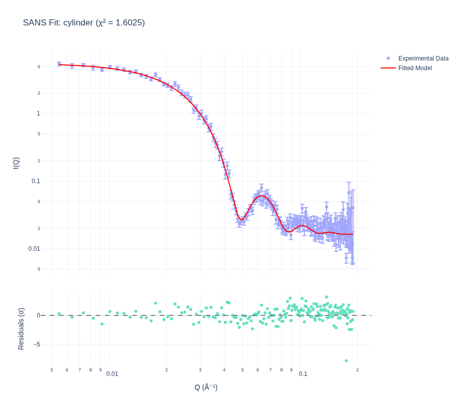
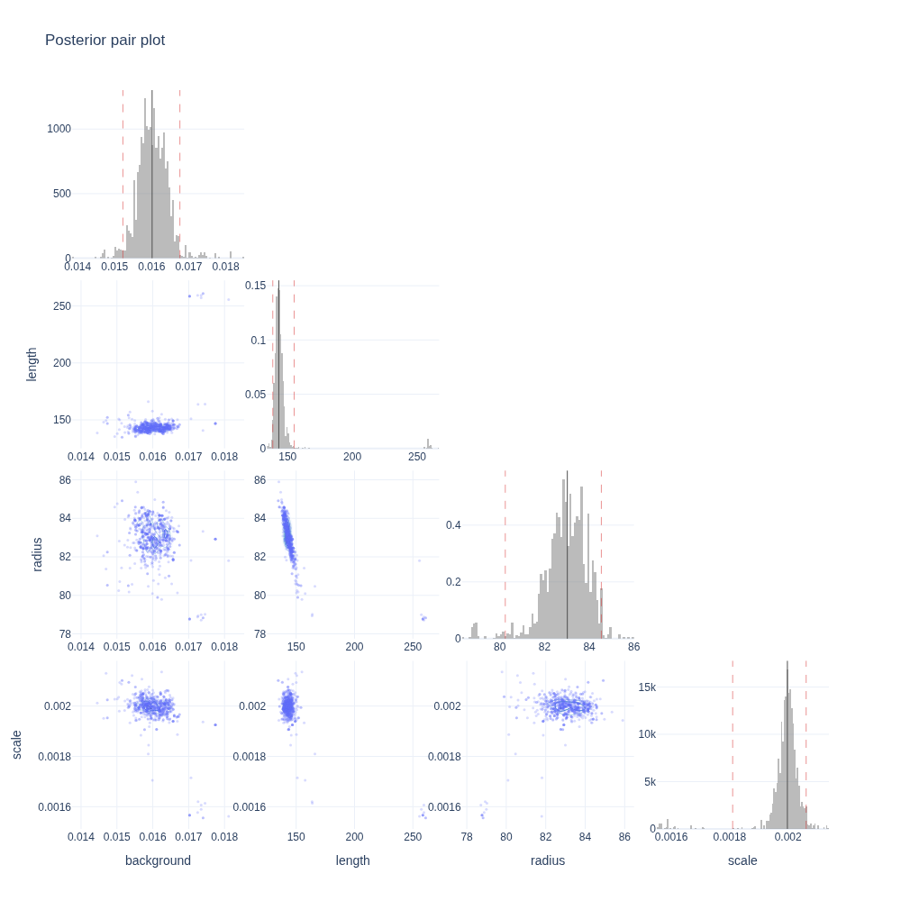
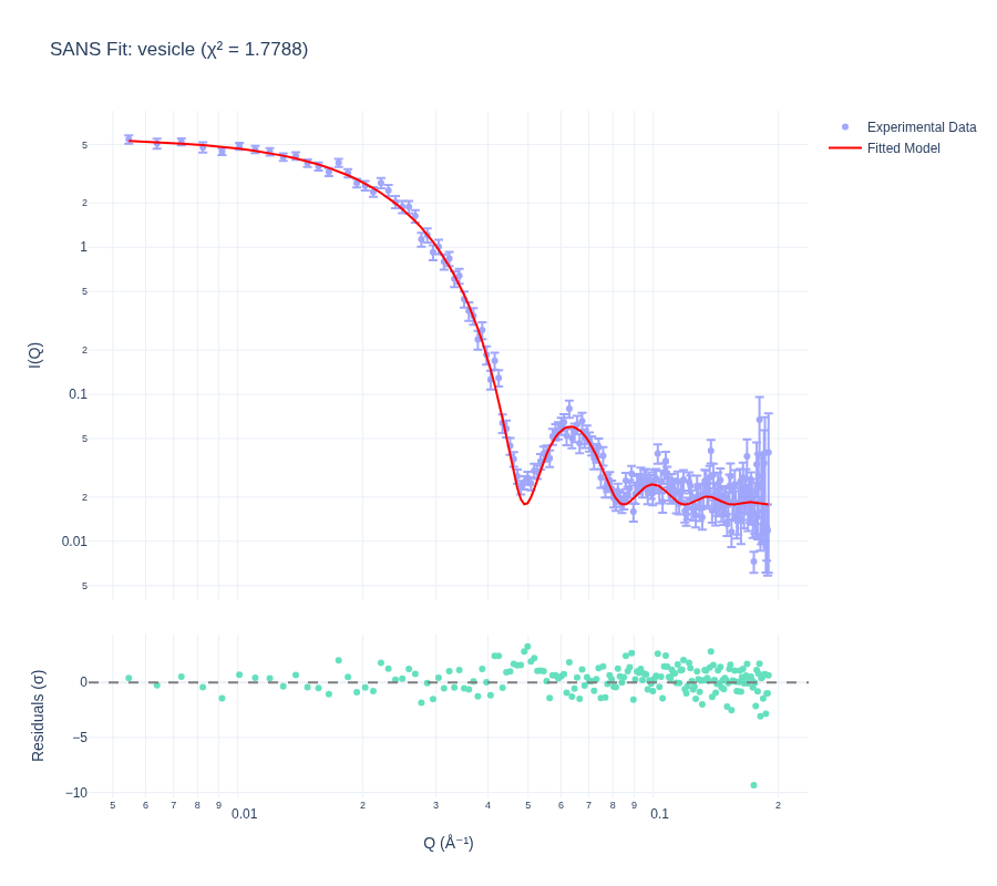
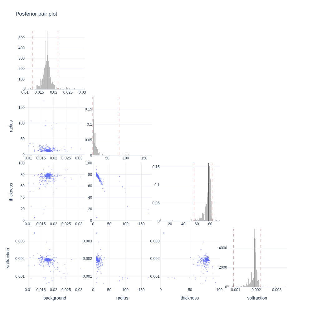
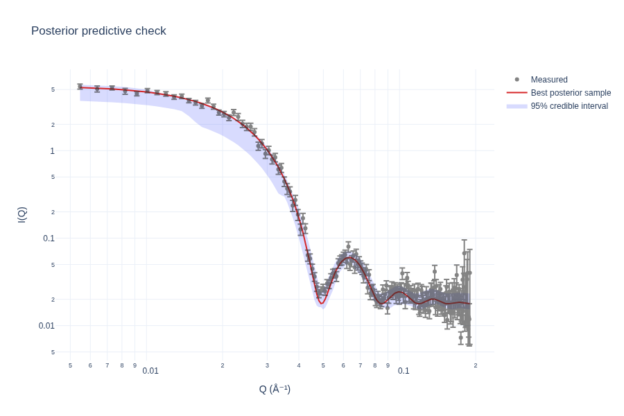
How do the different models compare? Do the fits, residuals, and posterior distributions single out one model as the best description of the data?
Consider also the physical plausibility of the fitted parameters: a model that fits well but requires unphysical parameter values should still be treated with suspicion.