Fitting QENS data#
Previously, some quasi-elastic neutron scattering (QENS) data has been simulated and reduced and can now be analysed with easyscience.
Before the analysis can begin, it is necessary to load the experimental data and check that it looks reasonable.
The data can be loaded with np.loadtxt as the data has been stored in a simple space-separated column file.
import numpy as np
import pandas as pd
import utils
filename = '../4-reduction/energy_transfer_QENS_unknown_quasi_elastic_many_neutrons.dat'
q, i, di = utils.load(filename)
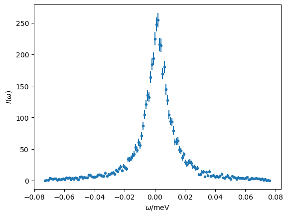
With the data read in, we can produce a quick plot.
import matplotlib.pyplot as plt

fig, ax = plt.subplots()
ax.errorbar(q, i, di, fmt='.')
ax.set(xlabel='$\\omega$/meV', ylabel='$I(\\omega)$')
plt.show()

The QENS data covers a slightly broader range than we want to investigate. Therefore, we will crop the data so that we are only using points between -0.06 and 0.06 meV.
sel = (q > -0.06) & (q < 0.06)
q, i, di = q[sel], i[sel], di[sel]
We now want to consider the mathematical model to be used in the analysis. QENS data is typically analysed by fitting a Lorentzian function to the data, which has the functional form
where \(A\) is a scale factor, \(\gamma\) is the half-width at half-maximum, and \(\omega_0\) is the centre offset.
Exercise 1: implement a Lorentzian function#
Write a function that implements Eqn. (3), called lorentzian.
Solution:
The instrument has a finite resolution, and to take this into account, the Lorentzian function must be convolved with this resolution. In our case, the resolution is a Gaussian distribution that is centred at zero with width, \(\sigma\). In real experiments there are ways to measure \(\sigma\), but for this project, we will simply model it.
from scipy.stats import norm

def intensity(omega):
    """
    The convolution of a Gaussian and the Lorentzian.

    :omega: the energy transfer values to calculate over.

    :return: intensity values.
    """
    gauss = norm(0, sigma.value).pdf(omega)
    gauss /= gauss.sum()
    return np.convolve(lorentzian(omega), gauss, 'same')
This means that there are a total of four parameters in our model.
Exercise 2: create fitting parameters#
Create four Parameter objects, for \(A\), \(\gamma\), \(\omega_0\), and \(\sigma\).
Each should have an initial value and a uniform prior distribution, based on the values given in Table 1.
Parameter |
Initial Value |
Min |
Max |
|---|---|---|---|
\(A\) |
10 |
1 |
100 |
\(\gamma\) |
8.0 × 10⁻³ |
1.0 × 10⁻⁴ |
1.0 × 10⁻² |
\(\omega_0\) |
1.0 × 10⁻³ |
-2.0 × 10⁻³ |
2.0 × 10⁻³ |
\(\sigma\) |
1.0 × 10⁻³ |
1.0 × 10⁻⁵ |
1.0 × 10⁻¹ |
Solution:
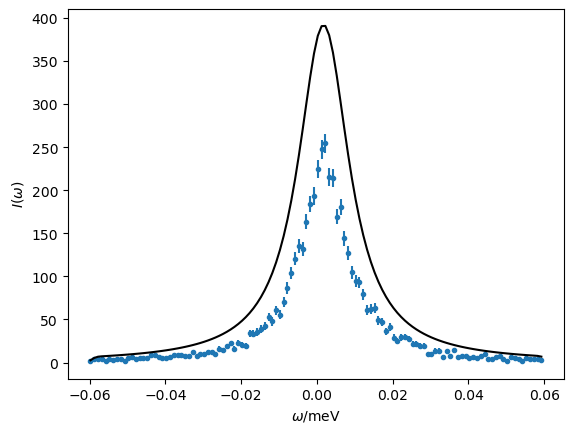
It is now possible to compare our model at the initial estimates to the simulated data.
fig, ax = plt.subplots()
ax.errorbar(q, i, di, fmt='.')
ax.plot(q, intensity(q), '-k', zorder=10)
ax.set(xlabel='$\\omega$/meV', ylabel='$I(\\omega)$')
plt.show()

Exercise 3: find maximum likelihood estimates#
Using easyscience, obtain maximum likelihood estimates for the four parameters of the model from comparison with the data.
Solution:
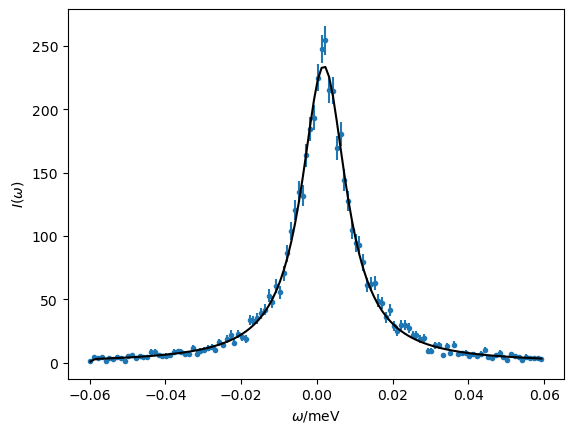
We can then plot the model and the data together as before and print the values of the parameters along with their uncertainties.
fig, ax = plt.subplots()
ax.errorbar(q, i, di, fmt='.')
ax.plot(q, intensity(q), '-k', zorder=10)
ax.set(xlabel='$\\omega$/meV', ylabel='$I(\\omega)$')
plt.show()

A, gamma, omega_0, sigma
(<Parameter 'A': 5.2217 ± 0.0601, bounds=[0.01:100.0]>,
 <Parameter 'gamma': 0.0070 ± 0.0001, bounds=[0.0001:0.01]>,
 <Parameter 'omega_0': 0.0011 ± 0.0001, bounds=[-0.002:0.002]>,
 <Parameter 'sigma': 0.0007 ± 0.0007, bounds=[1e-05:0.1]>)
Finally, we save the fit parameters to a CSV file.
utils.save_fit_params('qens_fit.csv', (A, gamma, omega_0, sigma))