Fitting SANS data#
Previously, some small angle neutron scattering (SANS) data has been simulated and reduced, and can now be analysed with easyscience.
Before the analysis can begin, it is necessary to load the experimental data and check that it looks reasonable.
The data can be loaded with np.loadtxt as the data has been stored in a simple space-separated column file.
import numpy as np
import utils
filename = '../4-reduction/sans_iofq.dat'
q, i, di = utils.load(filename)
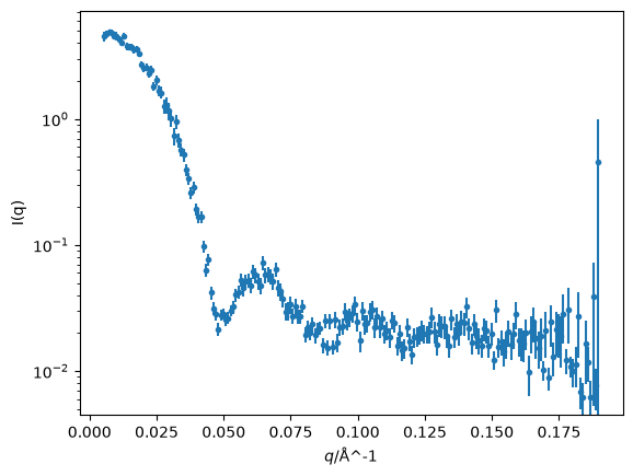
With the data read in, we can produce a quick plot.
import matplotlib.pyplot as plt

fig, ax = plt.subplots()
ax.errorbar(q, i, di, fmt='.')
ax.set(yscale='log', xlabel='$q$/Å^-1', ylabel='I(q)')
plt.show()
We now want to consider the mathematical model to be used in the analysis. There are SANS models a range of different systems, see for instance the models in SasView. However, initially, we will assume that our data has arisen from a spherical system.
The mathematical model for a sphere is
where \(\text{scale}\) is a scale factor, \(V\) is the volume of the sphere, \(\Delta \rho\) is the difference between the solvent and particle scattering length density, \(r\) is the radius of the sphere, \(\text{bkg}\) is a uniform background, and \(q\) is the q-vector that the intensity is being calculated for.
Exercise 1: simplify the expression#
The mathematical model described in Eqn. (4) has five parameters. What simple mathematical simplification can be performed to reduce this to four?
Solution:
Exercise 2: write a function that computes for the form factor of a sphere#
Four parameters is a suitable number for modelling. Therefore, we should write a function that implements your reduced dimensionality version of Eqn. (4).
Exercise 3: create fitting parameters#
Create four Parameter objects, for \(\text{scale}\), \(\Delta \rho\), \(r\), and \(\text{bkg}\).
Each should have an initial value and a uniform prior distribution based on the values given in Table 2, except for the \(\text{scale}\) which should be fixed to a value of 1.4 × 10⁻⁷.
Parameter |
Initial Value |
Min |
Max |
|---|---|---|---|
\(\text{scale}\) |
1.4 × 10⁻⁸ |
N/A |
N/A |
\(\Delta \rho\) |
3 |
0 |
10 |
\(r\) |
80 |
10 |
1000 |
\(\text{bkg}\) |
3.0 × 10⁻³ |
1.0 × 10⁻³ |
1.0 × 10⁻² |
Solution:
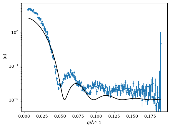
It is now possible to compare our model at the initial estimates to the simulated data.
fig, ax = plt.subplots()
ax.errorbar(q, i, di, fmt='.')
ax.plot(q, sphere(q), '-k', zorder=10)
ax.set(yscale='log', xlabel='$q$/Å^-1', ylabel='I(q)')
plt.show()
Exercise 4: find maximum likelihood estimates#
Using easyscience, obtain maximum likelihood estimates for the four parameters of the model from comparison with the data.
Solution:
We can then plot the model and the data together as before and print the values of the parameters along with their uncertainties.
fig, ax = plt.subplots()
ax.errorbar(q, i, di, fmt='.')
ax.plot(q, sphere(q), '-k', zorder=10)
ax.set(yscale='log', xlabel='$q$/Å^-1', ylabel='I(q)')
plt.show()
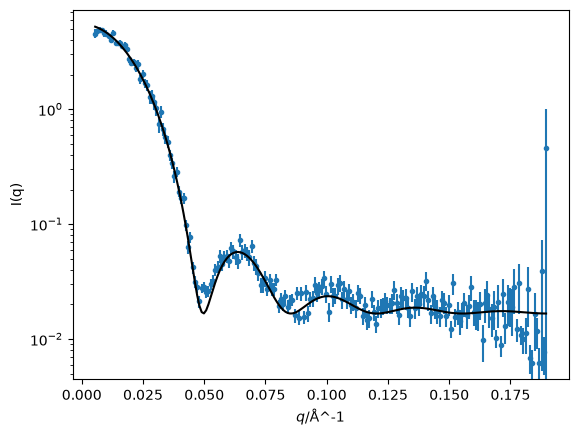
delta_rho, r, bkg
(<Parameter 'delta_rho': 3.5439 ± 0.0311, bounds=[0.0:10.0]>,
 <Parameter 'r': 90.5184 ± 0.3334, bounds=[0.0:1000.0]>,
 <Parameter 'bkg': 0.0167 ± 0.0004, bounds=[0.001:0.1]>)
Finally, we save the fit parameters to a CSV file.
utils.save_fit_params('sans_fit.csv', (delta_rho, r, bkg))