import mcstasscript as ms
import make_powder_instrument
from mcstasutils import plot
import quizlib
quiz = quizlib.Powder_Quiz()
Powder diffraction exercise#
In this notebook you will work with a McStas model of a simplified powder diffraction instrument. You will have to answer questions in the notebook by working with this model, both by running simulations and expanding the model. We will use the Python McStas API McStasScript to work with the instrument, you can find documentation here.
Get the instrument object#
First we need the McStas instrument object. Here it is retrieved from a local python function that generates it.
instrument = make_powder_instrument.make()
Investigate instrument#
The first task is to investigate the instrument object instrument using some of the available methods available on that object. Each method that show something about the instrument starts with the word show, so you can use tab to autocomplete in the cell to see the relevant methods.
In particular, look at what parameters are available and take a look at the instrument geometry.
Show code cell content
instrument.show_parameters()
       l_min                      = 0.5          // Minimum simulated
                                                     wavelength [AA]
       l_max                      = 4.0          // Maximum simulated
                                                     wavelength [AA]
int    n_pulses                   = 1            // Number of simulated pulses
       guide_curve_deg            = 1.0          //
       chopper_wavelength_center  = 2.5          // Center of wavelength band
                                                     [AA]
double frequency_multiplier       = 1            // [1] Chopper frequency as
                                                     multiple of source frequency
       detector_height            = 2.5          //
       sample_radius              = 0.01         //
       sample_height              = 0.05         //
string sample_choice              = "sample_Si"  //
Question 1#
Question about what is going on in the instrument model, checking for example how many choppers there are
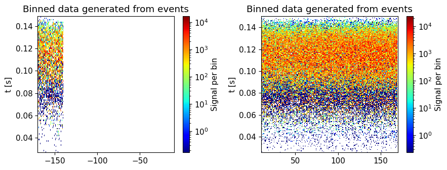
Run basic instrument for Si sample#
Run without pulse shaping chopper
instrument.get_component("chopper").set_WHEN("frequency_multiplier!=0") # code to remove chopper

instrument.set_parameters(sample_choice='"sample_Si"', frequency_multiplier=0, guide_curve_deg=0, detector_height=1.5)
instrument.settings(ncount=5.0e8, mpi=4, suppress_output=True, NeXus=True, output_path="powder_Si_initial")
data_initial = instrument.backengine()
plot(data_initial, orders_of_mag=5)
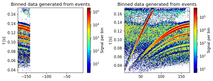
Add a chopper#
instrument.set_parameters(frequency_multiplier=1)
instrument.settings(output_path="powder_Si_with_chopper")
data_with_chopper = instrument.backengine()
plot(data_with_chopper, orders_of_mag=5)
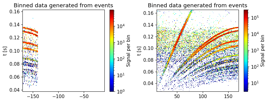
High-resolution chopper#
instrument.set_parameters(frequency_multiplier=3)
instrument.settings(output_path="powder_Si_high_resolution")
data_high_res = instrument.backengine()
plot(data_high_res, orders_of_mag=5)
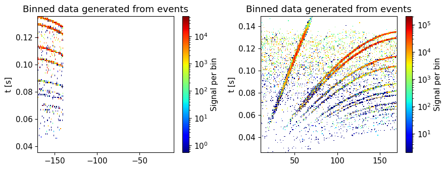
Run second (unknown) sample#
instrument.set_parameters(sample_choice='"sample_2"')
instrument.settings(output_path="powder_sample_2")

data_sample_2 = instrument.backengine()
plot(data_sample_2, orders_of_mag=5)
Run Vanadium sample#
instrument.set_parameters(sample_choice='"sample_Vanadium"')
instrument.settings(output_path="powder_vanadium")

data_vanadium = instrument.backengine()
plot(data_vanadium, orders_of_mag=5)