Powder diffraction data reduction#
This notebook will guide you through the data reduction for the powder diffraction experiment that you simulated with McStas yesterday.
The following is a basic outline of what this notebook will cover:
Loading the NeXus files that contain the data
Inspect/visualize the data contents
How to convert the raw event
time-of-arrivalcoordinate to something more useful (\(\lambda\), \(d\), …)Improve the estimate of neutron
time-of-flightSave the reduced data to disk, in a state that is ready for analysis/fitting.
import numpy as np
import scipp as sc
import plopp as pp
import utils
Process the run with a Si sample#
Load the NeXus file data#
folder = "../3-mcstas/powder_Si_high_resolution"

sample_si = utils.load_powder(folder)
The first way to inspect the data is to view the HTML representation of the loaded object.
Try to explore what is inside the data, and familiarize yourself with the different sections (Dimensions, Coordinates, Data).
sample_si
- events: 1426216
- position(events)vector3m[ 1.9190263 -0.2625 157.67299845], [ 1.9190263 -0.1875 157.67299845], ..., [ -3.21576924 -0.4875 159.2183965 ], [ -3.46803064 -0.1875 161.07197826]
Values:
array([[ 1.9190263 , -0.2625 , 157.67299845], [ 1.9190263 , -0.1875 , 157.67299845], [ 0.97940155, 0.5625 , 157.23982551], ..., [ -2.78600701, -0.1875 , 158.48147104], [ -3.21576924, -0.4875 , 159.2183965 ], [ -3.46803064, -0.1875 , 161.07197826]], shape=(1426216, 3)) - sample_position()vector3m[ 0. 0. 160.6]
Values:
array([ 0. , 0. , 160.6]) - sim_source_time(events)float64s0.000, 0.000, ..., 0.002, 0.004
Values:
array([0.00020381, 0.00020381, 0.00044506, ..., 0.00224308, 0.00209017, 0.00364308], shape=(1426216,)) - sim_speed(events)float64m/s1258.527, 1258.527, ..., 2125.108, 3249.229
Values:
array([1258.52717597, 1258.52717597, 1223.39680944, ..., 1778.23546527, 2125.10814501, 3249.22884854], shape=(1426216,)) - sim_wavelength(events)float64Å3.143, 3.143, ..., 1.862, 1.218
Values:
array([3.14338386, 3.14338386, 3.23364748, ..., 2.22469639, 1.86156833, 1.21753013], shape=(1426216,)) - source_position()vector3m[0. 0. 0.]
Values:
array([0., 0., 0.]) - time_origin()float64s0.0
Values:
array(0.) - toa(events)float64s0.131, 0.131, ..., 0.079, 0.054
Values:
array([0.13061412, 0.13061843, 0.13461796, ..., 0.09452714, 0.07936538, 0.05415352], shape=(1426216,)) - x(events)float64m1.919, 1.919, ..., -3.216, -3.468
Values:
array([ 1.9190263 , 1.9190263 , 0.97940155, ..., -2.78600701, -3.21576924, -3.46803064], shape=(1426216,)) - y(events)float64m-0.263, -0.188, ..., -0.487, -0.188
Values:
array([-0.2625, -0.1875, 0.5625, ..., -0.1875, -0.4875, -0.1875], shape=(1426216,)) - z(events)float64m157.673, 157.673, ..., 159.218, 161.072
Values:
array([157.67299845, 157.67299845, 157.23982551, ..., 158.48147104,
       159.2183965 , 161.07197826], shape=(1426216,))
- (events)float64counts0.547, 0.547, ..., 7.707e-08, 2.324σ = 0.547, 0.547, ..., 7.707e-08, 2.324
Values:
array([5.47429129e-01, 5.47429129e-01, 9.16157772e+00, ...,
       1.22053637e-06, 7.70708749e-08, 2.32399977e+00], shape=(1426216,))

Variances (σ²):
array([2.99678651e-01, 2.99678651e-01, 8.39345063e+01, ...,
       1.48970904e-12, 5.93991976e-15, 5.40097492e+00], shape=(1426216,))
Visualize the data#
Here is a 2D visualization of the neutron counts, histogrammed along the x and toadimensions:
sample_si.hist(x=200, toa=200).plot(norm="log", vmin=1.0e-2)

We can also visualize the events in 3D, which show the shape of the detector panels:
pp.scatter3d(sample_si[::20], pos='position', cbar=True, vmin=0.01, pixel_size=0.07)
Coordinate transformations#
The first step of this data reduction workflow is to convert the raw event coordinates (position, time-of-flight) to something physically meaningful such as wavelength (\(\lambda\)) or d-spacing (\(d\)).
Scipp has a dedicated method for this called transform_coords (see docs here).
We begin with a standard graph which describes how to compute e.g. the wavelength from the other coordinates in the raw data.
from scippneutron.conversion.graph.beamline import beamline
from scippneutron.conversion.graph.tof import kinematic

graph = {**beamline(scatter=True), **kinematic("tof")}

def compute_tof(toa, time_origin):
    return toa - time_origin

graph['tof'] = compute_tof
sc.show_graph(graph, simplified=True)

To compute the wavelength of all the events, we simply call transform_coords on our loaded data,
requesting the name of the coordinate we want in the output ("wavelength"),
as well as providing it the graph to be used to compute it (i.e. the one we defined just above).
This yields
si_wav = sample_si.transform_coords(["wavelength", "two_theta"], graph=graph)
si_wav
- events: 1426216
- L1()float64m160.6
Values:
array(160.6) - L2(events)float64m3.510, 3.505, ..., 3.534, 3.505
Values:
array([3.50982995, 3.50501872, 3.54491273, ..., 3.50501872, 3.5337878 , 3.50501872], shape=(1426216,)) - Ltotal(events)float64m164.110, 164.105, ..., 164.134, 164.105
Values:
array([164.10982995, 164.10501872, 164.14491273, ..., 164.10501872, 164.1337878 , 164.10501872], shape=(1426216,)) - incident_beam()vector3m[ 0. 0. 160.6]
Values:
array([ 0. , 0. , 160.6]) - position(events)vector3m[ 1.9190263 -0.2625 157.67299845], [ 1.9190263 -0.1875 157.67299845], ..., [ -3.21576924 -0.4875 159.2183965 ], [ -3.46803064 -0.1875 161.07197826]
Values:
array([[ 1.9190263 , -0.2625 , 157.67299845], [ 1.9190263 , -0.1875 , 157.67299845], [ 0.97940155, 0.5625 , 157.23982551], ..., [ -2.78600701, -0.1875 , 158.48147104], [ -3.21576924, -0.4875 , 159.2183965 ], [ -3.46803064, -0.1875 , 161.07197826]], shape=(1426216, 3)) - sample_position()vector3m[ 0. 0. 160.6]
Values:
array([ 0. , 0. , 160.6]) - scattered_beam(events)vector3m[ 1.9190263 -0.2625 -2.92700155], [ 1.9190263 -0.1875 -2.92700155], ..., [-3.21576924 -0.4875 -1.3816035 ], [-3.46803064 -0.1875 0.47197826]
Values:
array([[ 1.9190263 , -0.2625 , -2.92700155], [ 1.9190263 , -0.1875 , -2.92700155], [ 0.97940155, 0.5625 , -3.36017449], ..., [-2.78600701, -0.1875 , -2.11852896], [-3.21576924, -0.4875 , -1.3816035 ], [-3.46803064, -0.1875 , 0.47197826]], shape=(1426216, 3)) - sim_source_time(events)float64s0.000, 0.000, ..., 0.002, 0.004
Values:
array([0.00020381, 0.00020381, 0.00044506, ..., 0.00224308, 0.00209017, 0.00364308], shape=(1426216,)) - sim_speed(events)float64m/s1258.527, 1258.527, ..., 2125.108, 3249.229
Values:
array([1258.52717597, 1258.52717597, 1223.39680944, ..., 1778.23546527, 2125.10814501, 3249.22884854], shape=(1426216,)) - sim_wavelength(events)float64Å3.143, 3.143, ..., 1.862, 1.218
Values:
array([3.14338386, 3.14338386, 3.23364748, ..., 2.22469639, 1.86156833, 1.21753013], shape=(1426216,)) - source_position()vector3m[0. 0. 0.]
Values:
array([0., 0., 0.]) - time_origin()float64s0.0
Values:
array(0.) - toa(events)float64s0.131, 0.131, ..., 0.079, 0.054
Values:
array([0.13061412, 0.13061843, 0.13461796, ..., 0.09452714, 0.07936538, 0.05415352], shape=(1426216,)) - tof(events)float64s0.131, 0.131, ..., 0.079, 0.054
Values:
array([0.13061412, 0.13061843, 0.13461796, ..., 0.09452714, 0.07936538, 0.05415352], shape=(1426216,)) - two_theta(events)float64rad2.557, 2.559, ..., 1.972, 1.436
Values:
array([2.55701273, 2.55909034, 2.81733147, ..., 2.21984311, 1.9724811 , 1.43572818], shape=(1426216,)) - wavelength(events)float64Å3.149, 3.149, ..., 1.913, 1.305
Values:
array([3.14858595, 3.1487821 , 3.24440896, ..., 2.27873933, 1.91290385, 1.30546381], shape=(1426216,)) - x(events)float64m1.919, 1.919, ..., -3.216, -3.468
Values:
array([ 1.9190263 , 1.9190263 , 0.97940155, ..., -2.78600701, -3.21576924, -3.46803064], shape=(1426216,)) - y(events)float64m-0.263, -0.188, ..., -0.487, -0.188
Values:
array([-0.2625, -0.1875, 0.5625, ..., -0.1875, -0.4875, -0.1875], shape=(1426216,)) - z(events)float64m157.673, 157.673, ..., 159.218, 161.072
Values:
array([157.67299845, 157.67299845, 157.23982551, ..., 158.48147104,
       159.2183965 , 161.07197826], shape=(1426216,))
- (events)float64counts0.547, 0.547, ..., 7.707e-08, 2.324σ = 0.547, 0.547, ..., 7.707e-08, 2.324
Values:
array([5.47429129e-01, 5.47429129e-01, 9.16157772e+00, ...,
       1.22053637e-06, 7.70708749e-08, 2.32399977e+00], shape=(1426216,))

Variances (σ²):
array([2.99678651e-01, 2.99678651e-01, 8.39345063e+01, ...,
       1.48970904e-12, 5.93991976e-15, 5.40097492e+00], shape=(1426216,))
The result has a wavelength coordinate. We can also plot the result:
si_wav.hist(two_theta=128, wavelength=200).plot(norm='log', vmin=1.0e-3)

Exercise 1: convert raw data to d-spacing#
Instead of wavelength as in the example above, the task is now to convert the raw data to interplanar lattice spacing \(d\).
The transformation graph is missing the computation for \(d\) so you will have to add it in yourself. As a reminder, \(d\) is computed as follows
You have to:
create a function that computes \(d\)
add it to the graph with name “dspacing”
call
transform_coordsusing the new graph
Note that the graph already contains the necessary components to compute the scattering angle \(2 \theta\) (called two_theta in code).
Solution:
Show code cell content
def compute_d(two_theta, wavelength):
    return wavelength / (2 * sc.sin(two_theta / 2))


graph["dspacing"] = compute_d

# Show the updated graph
display(sc.show_graph(graph, simplified=True))

# Run the coordinate transformation
si_dspacing = sample_si.transform_coords("dspacing", graph=graph)
si_dspacing

- events: 1426216
- L1()float64m160.6
Values:
array(160.6) - L2(events)float64m3.510, 3.505, ..., 3.534, 3.505
Values:
array([3.50982995, 3.50501872, 3.54491273, ..., 3.50501872, 3.5337878 , 3.50501872], shape=(1426216,)) - Ltotal(events)float64m164.110, 164.105, ..., 164.134, 164.105
Values:
array([164.10982995, 164.10501872, 164.14491273, ..., 164.10501872, 164.1337878 , 164.10501872], shape=(1426216,)) - dspacing(events)float64Å1.644, 1.644, ..., 1.147, 0.992
Values:
array([1.64402161, 1.64361115, 1.64376142, ..., 1.27209525, 1.14688356, 0.99232951], shape=(1426216,)) - incident_beam()vector3m[ 0. 0. 160.6]
Values:
array([ 0. , 0. , 160.6]) - position(events)vector3m[ 1.9190263 -0.2625 157.67299845], [ 1.9190263 -0.1875 157.67299845], ..., [ -3.21576924 -0.4875 159.2183965 ], [ -3.46803064 -0.1875 161.07197826]
Values:
array([[ 1.9190263 , -0.2625 , 157.67299845], [ 1.9190263 , -0.1875 , 157.67299845], [ 0.97940155, 0.5625 , 157.23982551], ..., [ -2.78600701, -0.1875 , 158.48147104], [ -3.21576924, -0.4875 , 159.2183965 ], [ -3.46803064, -0.1875 , 161.07197826]], shape=(1426216, 3)) - sample_position()vector3m[ 0. 0. 160.6]
Values:
array([ 0. , 0. , 160.6]) - scattered_beam(events)vector3m[ 1.9190263 -0.2625 -2.92700155], [ 1.9190263 -0.1875 -2.92700155], ..., [-3.21576924 -0.4875 -1.3816035 ], [-3.46803064 -0.1875 0.47197826]
Values:
array([[ 1.9190263 , -0.2625 , -2.92700155], [ 1.9190263 , -0.1875 , -2.92700155], [ 0.97940155, 0.5625 , -3.36017449], ..., [-2.78600701, -0.1875 , -2.11852896], [-3.21576924, -0.4875 , -1.3816035 ], [-3.46803064, -0.1875 , 0.47197826]], shape=(1426216, 3)) - sim_source_time(events)float64s0.000, 0.000, ..., 0.002, 0.004
Values:
array([0.00020381, 0.00020381, 0.00044506, ..., 0.00224308, 0.00209017, 0.00364308], shape=(1426216,)) - sim_speed(events)float64m/s1258.527, 1258.527, ..., 2125.108, 3249.229
Values:
array([1258.52717597, 1258.52717597, 1223.39680944, ..., 1778.23546527, 2125.10814501, 3249.22884854], shape=(1426216,)) - sim_wavelength(events)float64Å3.143, 3.143, ..., 1.862, 1.218
Values:
array([3.14338386, 3.14338386, 3.23364748, ..., 2.22469639, 1.86156833, 1.21753013], shape=(1426216,)) - source_position()vector3m[0. 0. 0.]
Values:
array([0., 0., 0.]) - time_origin()float64s0.0
Values:
array(0.) - toa(events)float64s0.131, 0.131, ..., 0.079, 0.054
Values:
array([0.13061412, 0.13061843, 0.13461796, ..., 0.09452714, 0.07936538, 0.05415352], shape=(1426216,)) - tof(events)float64s0.131, 0.131, ..., 0.079, 0.054
Values:
array([0.13061412, 0.13061843, 0.13461796, ..., 0.09452714, 0.07936538, 0.05415352], shape=(1426216,)) - two_theta(events)float64rad2.557, 2.559, ..., 1.972, 1.436
Values:
array([2.55701273, 2.55909034, 2.81733147, ..., 2.21984311, 1.9724811 , 1.43572818], shape=(1426216,)) - wavelength(events)float64Å3.149, 3.149, ..., 1.913, 1.305
Values:
array([3.14858595, 3.1487821 , 3.24440896, ..., 2.27873933, 1.91290385, 1.30546381], shape=(1426216,)) - x(events)float64m1.919, 1.919, ..., -3.216, -3.468
Values:
array([ 1.9190263 , 1.9190263 , 0.97940155, ..., -2.78600701, -3.21576924, -3.46803064], shape=(1426216,)) - y(events)float64m-0.263, -0.188, ..., -0.487, -0.188
Values:
array([-0.2625, -0.1875, 0.5625, ..., -0.1875, -0.4875, -0.1875], shape=(1426216,)) - z(events)float64m157.673, 157.673, ..., 159.218, 161.072
Values:
array([157.67299845, 157.67299845, 157.23982551, ..., 158.48147104,
       159.2183965 , 161.07197826], shape=(1426216,))
- (events)float64counts0.547, 0.547, ..., 7.707e-08, 2.324σ = 0.547, 0.547, ..., 7.707e-08, 2.324
Values:
array([5.47429129e-01, 5.47429129e-01, 9.16157772e+00, ...,
       1.22053637e-06, 7.70708749e-08, 2.32399977e+00], shape=(1426216,))

Variances (σ²):
array([2.99678651e-01, 2.99678651e-01, 8.39345063e+01, ...,
       1.48970904e-12, 5.93991976e-15, 5.40097492e+00], shape=(1426216,))
Histogram the data in d-spacing#
The final step in processing the sample run is to histogram the data into \(d\) bins.
dbins = sc.linspace ('dspacing', 0.5, 2.5, 2001, unit='angstrom')
ntheta = 128

si_dspacing_hist = si_dspacing.hist(two_theta=ntheta, dspacing=dbins)
si_dspacing_hist.plot(norm='log', vmin=1.0e-3)

si_dspacing_hist.sum('two_theta').plot()

Exercise 2: Correct the time-of-flight#
Time-of-flight at a long-pulsed source#
The time-of-flight of a neutron is typically not known from experimental measurements.
The only two parameters that we are able to record are usually the time at which the pulse was emitted (named time_origin in our dataset),
and the timestamp when a neutron was detected by a detector pixel (named toa, standing for time-of-arrival).
The difference between these two times is commonly used to compute an approximate time-of-flight. This approximation performs well at neutron sources with a short pulse, where it is satisfactory to assume that all neutrons left the source at the same time.
At a long-pulsed source (lasting a few milliseconds) such as ESS, with high-precision instruments, this approximation is no longer valid.
This is in fact the reason why in the \(2\theta\) vs d-spacing plot, the bright lines appear curved while they should in reality be vertical.
In the following exercise, we will add a correction to our time-of-flight computation to improve our results.
Finding a new time-distance origin#
One way to look at the problem is to visualize the paths of each neutron that made it to the detector, on a time-distance diagram.
The neutrons begin at the source (bottom left), travel along the guide, go through the chopper, and finally arrive at the detectors (top).
from powder_utils import time_distance_diagram

time_distance_diagram(si_wav)
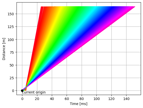
As the figure above illustrates,
the current time-of-flight computation (tof = toa - time_origin) assumes that all neutrons were born at \(t = 0\) (black dot).
This is clearly not the case from looking at the neutron tracks.
Exercise: find a new origin#
Inspect the time-distance diagram and try to find a point which would be a better representation of a common origin for all tracks.
Set the origin as coordinates on the original data (hint: you will need to update the
source_positionandtime_origincoordinates).Compute wavelength/d-spacing again.
Solution:
Show code cell content
better = sample_si.copy(deep=False)

# Read off the plot that the lines cross as they go through the chopper:
# time=5.53, distance=6.5 (approximately)
better.coords['source_position'] = sc.vector([0, 0, 6.5], unit='m')
better.coords['time_origin'] = sc.scalar(5.53, unit='ms').to(unit='s')

better_dspacing = better.transform_coords("dspacing", graph=graph)
better_dspacing
- events: 1426216
- L1()float64m154.1
Values:
array(154.1) - L2(events)float64m3.510, 3.505, ..., 3.534, 3.505
Values:
array([3.50982995, 3.50501872, 3.54491273, ..., 3.50501872, 3.5337878 , 3.50501872], shape=(1426216,)) - Ltotal(events)float64m157.610, 157.605, ..., 157.634, 157.605
Values:
array([157.60982995, 157.60501872, 157.64491273, ..., 157.60501872, 157.6337878 , 157.60501872], shape=(1426216,)) - dspacing(events)float64Å1.639, 1.639, ..., 1.111, 0.928
Values:
array([1.63934691, 1.63894199, 1.64122825, ..., 1.24707043, 1.11096768, 0.92774245], shape=(1426216,)) - incident_beam()vector3m[ 0. 0. 154.1]
Values:
array([ 0. , 0. , 154.1]) - position(events)vector3m[ 1.9190263 -0.2625 157.67299845], [ 1.9190263 -0.1875 157.67299845], ..., [ -3.21576924 -0.4875 159.2183965 ], [ -3.46803064 -0.1875 161.07197826]
Values:
array([[ 1.9190263 , -0.2625 , 157.67299845], [ 1.9190263 , -0.1875 , 157.67299845], [ 0.97940155, 0.5625 , 157.23982551], ..., [ -2.78600701, -0.1875 , 158.48147104], [ -3.21576924, -0.4875 , 159.2183965 ], [ -3.46803064, -0.1875 , 161.07197826]], shape=(1426216, 3)) - sample_position()vector3m[ 0. 0. 160.6]
Values:
array([ 0. , 0. , 160.6]) - scattered_beam(events)vector3m[ 1.9190263 -0.2625 -2.92700155], [ 1.9190263 -0.1875 -2.92700155], ..., [-3.21576924 -0.4875 -1.3816035 ], [-3.46803064 -0.1875 0.47197826]
Values:
array([[ 1.9190263 , -0.2625 , -2.92700155], [ 1.9190263 , -0.1875 , -2.92700155], [ 0.97940155, 0.5625 , -3.36017449], ..., [-2.78600701, -0.1875 , -2.11852896], [-3.21576924, -0.4875 , -1.3816035 ], [-3.46803064, -0.1875 , 0.47197826]], shape=(1426216, 3)) - sim_source_time(events)float64s0.000, 0.000, ..., 0.002, 0.004
Values:
array([0.00020381, 0.00020381, 0.00044506, ..., 0.00224308, 0.00209017, 0.00364308], shape=(1426216,)) - sim_speed(events)float64m/s1258.527, 1258.527, ..., 2125.108, 3249.229
Values:
array([1258.52717597, 1258.52717597, 1223.39680944, ..., 1778.23546527, 2125.10814501, 3249.22884854], shape=(1426216,)) - sim_wavelength(events)float64Å3.143, 3.143, ..., 1.862, 1.218
Values:
array([3.14338386, 3.14338386, 3.23364748, ..., 2.22469639, 1.86156833, 1.21753013], shape=(1426216,)) - source_position()vector3m[0. 0. 6.5]
Values:
array([0. , 0. , 6.5]) - time_origin()float64s0.00553
Values:
array(0.00553) - toa(events)float64s0.131, 0.131, ..., 0.079, 0.054
Values:
array([0.13061412, 0.13061843, 0.13461796, ..., 0.09452714, 0.07936538, 0.05415352], shape=(1426216,)) - tof(events)float64s0.125, 0.125, ..., 0.074, 0.049
Values:
array([0.12508412, 0.12508843, 0.12908796, ..., 0.08899714, 0.07383538, 0.04862352], shape=(1426216,)) - two_theta(events)float64rad2.557, 2.559, ..., 1.972, 1.436
Values:
array([2.55701273, 2.55909034, 2.81733147, ..., 2.21984311, 1.9724811 , 1.43572818], shape=(1426216,)) - wavelength(events)float64Å3.140, 3.140, ..., 1.853, 1.220
Values:
array([3.13963308, 3.13983705, 3.23940905, ..., 2.23391168, 1.85299922, 1.220496 ], shape=(1426216,)) - x(events)float64m1.919, 1.919, ..., -3.216, -3.468
Values:
array([ 1.9190263 , 1.9190263 , 0.97940155, ..., -2.78600701, -3.21576924, -3.46803064], shape=(1426216,)) - y(events)float64m-0.263, -0.188, ..., -0.487, -0.188
Values:
array([-0.2625, -0.1875, 0.5625, ..., -0.1875, -0.4875, -0.1875], shape=(1426216,)) - z(events)float64m157.673, 157.673, ..., 159.218, 161.072
Values:
array([157.67299845, 157.67299845, 157.23982551, ..., 158.48147104,
       159.2183965 , 161.07197826], shape=(1426216,))
- (events)float64counts0.547, 0.547, ..., 7.707e-08, 2.324σ = 0.547, 0.547, ..., 7.707e-08, 2.324
Values:
array([5.47429129e-01, 5.47429129e-01, 9.16157772e+00, ...,
       1.22053637e-06, 7.70708749e-08, 2.32399977e+00], shape=(1426216,))

Variances (σ²):
array([2.99678651e-01, 2.99678651e-01, 8.39345063e+01, ...,
       1.48970904e-12, 5.93991976e-15, 5.40097492e+00], shape=(1426216,))
better_dspacing.hist(two_theta=ntheta, dspacing=dbins).plot(norm='log', vmin=1.0e-3)

pp.plot({'original': si_dspacing_hist.sum('two_theta'),
         'improved': better_dspacing.hist(two_theta=ntheta, dspacing=dbins).sum('two_theta')})

Process the Vanadium run#
folder = "../3-mcstas/powder_vanadium"

sample_van = utils.load_powder(folder)

# Read off the plot that the lines cross as they go through the chopper:
# time=5.53, distance=6.5 (approximately)
sample_van.coords['source_position'] = sc.vector([0, 0, 6.5], unit='m')
sample_van.coords['time_origin'] = sc.scalar(5.53, unit='ms').to(unit='s')

van_dspacing = sample_van.transform_coords("dspacing", graph=graph)
van_dspacing.hist(two_theta=ntheta, dspacing=dbins).plot(norm='log', vmin=1.0e-3)

Normalize by Vanadium#
num = better_dspacing.hist(two_theta=ntheta, dspacing=dbins)
den = van_dspacing.hist(two_theta=num.coords['two_theta'], dspacing=dbins)
# Smooth the Vanadium run
from scipp.scipy.ndimage import gaussian_filter

smooth_vana = gaussian_filter(
    sc.values(den.sum('two_theta')),
    sigma=sc.scalar(0.02, unit='angstrom')
)

pp.plot({'orig': den.sum('two_theta'),
         'smooth': smooth_vana},
        title='Vanadium - smoothed')

normed = (num.sum('two_theta') / smooth_vana)

normed.plot()

Save to disk#
average_l = better_dspacing.coords["Ltotal"].mean()
average_two_theta = better_dspacing.coords["two_theta"].mean()
difc = sc.to_unit(
    2
    * sc.constants.m_n
    / sc.constants.h
    * average_l
    * sc.sin(0.5 * average_two_theta),
    unit='us / angstrom',
)

average_l , sc.to_unit(average_two_theta, 'deg'), difc
(<scipp.Variable> ()    float64              [m]  157.626,
 <scipp.Variable> ()    float64            [deg]  100.719,
 <scipp.Variable> ()    float64         [10N/mW]  61365.3)
from scippneutron.io import save_xye

result_si = normed.copy(deep=False)
result_si.coords["tof"] = (sc.midpoints(result_si.coords["dspacing"]) * difc).to(unit='us')

save_xye("powder_reduced_Si.xye", result_si.rename_dims(dspacing='tof'),
         header=f"DIFC = {difc.to(unit='us/angstrom').value} [µ/Å] L = {average_l.value} [m] two_theta = {sc.to_unit(average_two_theta, 'deg').value} [deg]\ntof [µs]               Y [counts]               E [counts]")
Process and normalize unknown sample#
folder = "../3-mcstas/powder_sample_2"

unknown = utils.load_powder(folder)

# Read off the plot that the lines cross as they go through the chopper:
# time=5.53, distance=6.5 (approximately)
unknown.coords['source_position'] = sc.vector([0, 0, 6.5], unit='m')
unknown.coords['time_origin'] = sc.scalar(5.53, unit='ms').to(unit='s')

unknown_dspacing = unknown.transform_coords("dspacing", graph=graph)
unknown_dspacing.hist(two_theta=ntheta, dspacing=dbins).plot(norm='log', vmin=1.0e-3)

# Normalize
unknown_num = unknown_dspacing.hist(two_theta=den.coords['two_theta'], dspacing=dbins)

unknown_normed = (unknown_num.sum('two_theta') / smooth_vana)

unknown_normed.plot()

average_l = unknown_dspacing.coords["Ltotal"].mean()
average_two_theta = unknown_dspacing.coords["two_theta"].mean()
difc = sc.to_unit(
    2
    * sc.constants.m_n
    / sc.constants.h
    * average_l
    * sc.sin(0.5 * average_two_theta),
    unit='us / angstrom',
)
average_l , sc.to_unit(average_two_theta, 'deg'), difc
(<scipp.Variable> ()    float64              [m]  157.626,
 <scipp.Variable> ()    float64            [deg]  94.7832,
 <scipp.Variable> ()    float64         [10N/mW]  58650.9)
Save to disk#
result_unknown = unknown_normed.copy(deep=False)
result_unknown.coords["tof"] = (sc.midpoints(result_unknown.coords["dspacing"]) * difc).to(unit='us')

save_xye("powder_reduced_unknown.xye", result_unknown.rename_dims(dspacing='tof'),
         header=f"DIFC = {difc.to(unit='us/angstrom').value} [µ/Å] L = {average_l.value} [m] two_theta = {sc.to_unit(average_two_theta, 'deg').value} [deg]\ntof [µs]               Y [counts]               E [counts]")